
Disclaimer: This blog post was written by an external contributor about techniques for validating marketing mix models using cross-validation. The approach laid out in this document is not reflective of how Recast approaches model validation. The actual model specification can be found in the technical model specification.
You’ve spent countless hours building a marketing mix model with the goal of reallocating millions of dollars in marketing spend. How can you be sure that your model is not completely misguided? What can you do to build trust so you can have a reasonable level of confidence in the decisions resulting from your model?
It has been more than twenty years since Leo Breiman wrote his famous “Statistical Modelling: The Two Cultures” paper. Breiman wrote that “there are two cultures in the use of statistical modeling to reach conclusions from data.”
Almost every first year business student is inducted into the “data modeling culture”, or traditional frequentist statistics. Whereas modern applications of Machine Learning, such as image recognition and AutoML, are firmly in the “algorithmic modeling culture”.
The data modeling culture uses goodness-of-fit tests and residual examination to validate models. Statistical tests on model parameters are goodness-of-fit tests. For example, t-tests on regression coefficients. Residual examination includes plotting the in-sample residuals and looking for patterns. Adjusted R2 is also calculated from the model residuals. The model is viewed as an estimate of the underlying data generating process. Out-of-sample validation – testing the model against unseen data – is often an afterthought, if it’s done at all.
Goodness-of-fit tests and residual examination were useful and appropriate for the scenarios for which they were developed. However, they are probably being mis-applied in modern settings. Here are two quotes from Breiman.
“Work by Bickel, Ritov and Stoker (2001) shows that goodness-of-fit tests have very little power unless the direction of the alternative is precisely specified. The implication is that omnibus goodness-of-fit tests, which test in many directions simultaneously, have little power, and will not reject until the lack of fit is extreme.” – Leo Breiman, Statistical Modelling: The Two Cultures
“In a discussion after a presentation of residual analysis in a seminar at Berkeley in 1993, William Cleveland, one of the fathers of residual analysis, admitted that it could not uncover lack of fit in more than four to five dimensions.” – Leo Breiman, Statistical Modelling: The Two Cultures
The algorithmic modeling culture is accustomed to high-variance models, in which the risk of overfitting to the data abound. Hence, the algorithmic modeling culture uses out-of-sample performance to validate models. There is no reliance on traditional statistical tests in the algorithmic modeling culture.
Algorithmic models are not entirely the black boxes that the mainstream tech media portray them to be. For example, LIME is a modern method for interpreting algorithmic models. Back in Breiman’s time, statisticians would fit interpretable surrogate models to the outputs of black box models. Most gradient boosted tree packages can produce partial dependence plots as part of their standard output. Also Bayesian models such as used at Recast can be highly interpretable.
The modern Marketing Mix Model borrows from both cultures. The company has some control over the data generating process. It controls its marketing spend on various channels. Bayesian Marketing Mix Models estimate the entire posterior distribution of model parameters. The estimated effects of each marketing channel have a range, rather than a point estimate and a hard “accept/reject” decision. Modern Marketing Mix Models are evaluated on their out-of-sample performance, rather than goodness-of-fit tests.
Marketing Mix data is time series data. Our dependent variable is usually Sales at time t. Our independent variables are expenditure on various marketing channels at time t, as well as lagged observations. Most internet tutorials focus on cross-validation of cross-sectional data, where each observation is independent of other observations. In time series data, each observation is related to previous observations. Cross-sectional cross-validation methods randomly split the dataset. When splitting time series data, we need to preserve its order in time.
Cross-Validation for Time Series Models
The right way to split your time series data for model validation

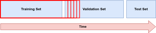
The most basic split is easy to implement and it gives us a starting point for explaining the more advanced time series cross-validation setup. Examine the diagram above. The training, validation, and test datasets are sequential in order, rather than chosen at random like they would be with normal machine learning: this is essential for time series data so there’s no potential for information to bleed through into the training process.
We train the model on the earliest available data, the training set. The next set of observations, in chronological order (say for example, the final 30 days of the dataset), is the validation set. After training the model on the training set, we evaluate its performance on the validation set. We compare the performance on the validation set across different candidate models and different sets of hyperparameters.
Next, we concatenate our training and validation sets and re-train our final model. The final model is the one candidate model that we selected by evaluating performance on the validation set. We use the subset of features and hyperparameter settings that we selected by optimizing on the validation set.
We expect that the performance on the test set will be worse than on the validation set – because we optimized for the validation set. We check to make sure that the difference is not too big and that the model is still fit for purpose.
A more advanced cross-validation setup
A more advanced cross-validation setup involves several iterations of walking forward. On the first iteration, we train our model on the training set and predict for h periods ahead. We then evaluate our performance on the first h periods of the validation set. On the next iteration, we expand our training set, re-train our model, predict another h periods ahead, and then evaluate our performance on the validation set. We iterate until we have used up the whole validation set.
I have come across several names for this process: “walk forward”, “rolling window”, “expanding window”, and a new name is likely just around the corner.
When cross-validating cross-sectional data, you will have one prediction per fold. You can stack all of the folds and compute a single performance metric. However, in walk forward cross-validation, your folds or prediction windows might overlap. You will have a vector of performance metrics – one for each overlapping window. How should we combine these iteration metrics into a single number, so that we can compare candidate models?
The simplest option is to take the average and then choose the best candidate model according to a single number. You can also examine the distribution of the performance metrics – are there any big outliers? You can also plot the series of metrics as a time series – is there a point in time where the model performs particularly badly?
Error Metrics for Regression Problems
We have mentioned performance metrics as an abstract term. Now here are some actual performance metrics that you can use for evaluating any real valued predictions.
Our one-step-ahead forecast error, at time t, is defined as:

Where y at time t is what we are trying to predict, and ŷt are the predictions from the model.

MAE is easy to calculate and easy to interpret.
Squared-Error Based Metrics


Meta’s Robyn MMM package uses NRMSE.
Percentage-Error Based Metrics

MAPE is asymmetric. Having yt in the denominator means that it will penalize positive errors more than negative errors. If we were to replace yt with yt, then it would penalize smaller values of yt more than higher values of yt. There is also a symmetric MAPE.

A disadvantage of both MAPE and sMAPE is that they don’t perform very well when yt is close to zero, and they are undefined when the denominator is exactly zero.
Uber’s Orbit MMM package uses sMAPE.
A Scaled-Error Based Metric
Mean Absolute Scaled Error (MASE) compares the error to the MAE of the naive or random walk model on the training set. The rationale for using the training set data is to account for the case when the validation set only has a handful of observations.

where yi is the ith observation in the training set.

Best Practices At Recast
Recast uses a 30 day test set to check each model before presenting to clients. They simulate how the model will be used – predicting the next few months of sales, given expenditure on various channels, to make budgeting decisions.
As well as being accurate, a Marketing Mix Model also needs to be plausible. The Recast team always sense-check their models. For example, they check to make sure that there aren’t any unrealistic coefficients. An obvious error would if most credit gets assigned to one small marketing channel. Another error, which suggests multicollinearity, is to see two variables with almost equal and opposite coefficients.
It’s also important to check the data for errors before modeling. Huge spikes in sales on certain days could be special events (eg. boxing day). Or they could be double counting errors or transactions over several days being recorded as having occurred on a single day.
Hopefully this article has expanded your data science toolbox – and helped you succeed in your career. Subscribe to the Recast newsletter to receive the latest articles as they come out.
References
- Breiman, L., 2001, Statistical Modelling: The Two Cultures, https://projecteuclid.org/journals/statistical-science/volume-16/issue-3/Statistical-Modeling–The-Two-Cultures-with-comments-and-a/10.1214/ss/1009213726.full, accessed on 2023-02-08
- Hyndman et al., 2008, Forecasting with Exponential Smooothing, Springer Verlag
- NRMSE, https://www.statisticshowto.com/nrmse/, accessed on 2023-02-08