
You can boost revenue by scientifically optimizing your marketing spend. What could go wrong? Statistical mistakes could de-optimize your marketing spend. It will seem very “scientific” while you are doing it. You will feel very good about it until senior management notices the drop in sales – and subjects you to extreme scrutiny.
One way your analysis could be ruined is by confounding variables. We’ll use the following scenario to illustrate what confounding variables are, and how they can ruin your regression analysis. In this scenario, our company is a large online store. The online store has several departments – including clothing and homeware. Customer acquisition and customer retention is managed by separate teams.
Our Scenario – Two teams that should have been talking to each other
The Acquisition Team – Building a Marketing Mix Model
The acquisition team wants to estimate the impact of each of their marketing channels – Paid Search, Display, and Paid Social.
The Head of Acquisition has a lot of discretion as to how the budget is allocated amongst Paid Search, Display, and Paid Social. The team runs various campaigns throughout the year, including a high spending Christmas campaign. Sometimes acquisition advertising spend is discretionarily reduced and at other times it is discretionarily increased.
The acquisition team has had a lot of trouble evaluating the ROI of their marketing spend. This time, the acquisition team is building a Marketing Mix Model. The Head of Acquisition hears that some additional variability in spend will help the regression analysis. Hence he has decided to increase the spend on Paid Search for a few weeks.
Aside from senior management, no other team in the company is briefed on what the acquisition team does day to day. No other team is aware of how the spend on Paid Search, Display, and Paid Social fluctuates.
The Retention Team – Evaluating their Cross-Sell Campaign
The retention team sends retention offers through their CRM system. The retention team is trialing the company’s first cross-sell model. Customers receive emails that recommend products in departments that they rarely buy from. For example, they recommend homeware items to customers who primarily buy clothing.
The cross-sell campaign was (coincidentally) started in the same week that the acquisition team increased their Paid Search budget. Aside from senior management, no other team in the company is aware of this cross-sell campaign. No other team is aware of exactly what emails are sent to customers, and when they are sent.
Acquisition Team – Gets Unstable Regression Results
The acquisition team’s data analyst runs the Marketing Mix Model model after the increase in Paid Search spend. The model is a Linear Regression. The dependent variable is sales revenue per day. The independent variables are the spend on the various channels that the acquisition team is aware of, and a seasonal term. All of the effects in the model are assumed to be linear because that’s what the analyst knows.
The data analyst estimates the following regression equation.
The analyst concludes that the increased spend on Paid Search leads to increased sales revenue. The analyst confidently writes “statistically significant at the 5% level” in her slide deck.
In the following week, the analyst re-runs the model. The budget for Paid Search has now returned to previous levels. In this iteration of the regression model, the coefficient on Paid Search is “not statistically significant at the 5% level”. It’s still positive, but the p-value is way too high. The analyst is bewildered to learn that p-values can fluctuate from week to week. She wonders if something can be “statistically significant at the 37% level?”.
Retention Team – Ignores unobserved factors
The retention team used a process that they called “A/B Testing” in their slide deck. First, they identified a segment of customers who were “primarily one department shoppers”. 90% of this segment received a series of cross-sell emails. The other 10% were held out as the “control group” and did not receive any emails at all. The uplift calculation process compared the average sales per customer between the “target” and “control” groups.
Initially, the retention team concluded that the cross-sell campaign produced positive uplift. However, the retention team was not aware that the acquisition team runs a remarketing campaign.
A few weeks later, the acquisition team increased their budget for remarketing to people who had previously visited the online store. The retention team was not aware that existing customers were seeing more Display ads, more often. The calculated uplift on the cross-sell campaign reduced dramatically. Nobody in the retention team had any idea that there could have been any unobserved factors.
So what are confounding variables?
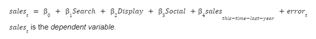
A confounding variable affects the dependent variable but is not included in the analysis. For example, the acquisition team’s attribution model is the following regression equation.

The spend on Paid Search, Display and Paid Social are independent variables in the regression. So is the seasonal term sales this-time-last-year. A regression model uses the independent variables to explain the dependent variable.
The retention team’s cross-sell campaign is a confounding variable for the acquisition team’s Marketing Mix Model. The cross-sell campaign affects sales, but the acquisition team is not aware of it.
The model might think the increased spend on Paid Search leads to a strong increase in sales revenue, when some credit should go to the cross-sell campaign. We are not actually sure exactly how much credit should be given to the cross-sell campaign and how much should go to the increased spend on Paid Search.
The evaluation of the cross-sell campaign is confounded by the impact of sending an email. Because the control group in the cross-sell campaign does not receive an email at all. The measure of campaign performance is the average change in sales per customer – rather than “breadth” of products bought. The increased sales might have been caused by the email – whether the cross-sell recommendations were relevant or not.
The increased remarketing spend was also a confounding variable in the analysis of the cross-sell campaign. The increased remarketing budget increased the chance that a customer in the “control” group of the cross-sell campaign would receive a marketing message from our company.
What could have the acquisition team done better?
The two marketing teams need to be aware of what the other is doing. Ideally, all data should be accessible in one place. Even without a “customer 360” platform, the acquisition team would have been able to account for the retention team’s activities with a few data extracts.
The acquisition team’s Marketing Mix Model did not account for the effect of the cross-sell campaign. Since the cross-sell campaign overlaps with the increased spend on Paid Search, it’s not clear how much uplift to attribute to each one. They should both be covariates in the regression.
The Marketing Mix Modeling process should also experiment with non-linear functions of the independent variables. Because increased spending on certain channels might bring diminishing returns after a certain level of saturation. Non-linear functions of spend can explicitly encode this into the model.
End-to-end regression analysis includes the analysis of the regression errors, also known as residuals or disturbances. Regression errors are the difference between the observed values, y, and the predicted values, y. Our data analyst could use a spreadsheet to calculate the errors from the Marketing Mix Model. She would just subtract the column with the sales figure predicted by the regression equation, from the column with the actual observed sales.
A quick, informal way to analyze regression errors would be to plot the errors versus time and look for any obvious patterns. Patterns in regression residuals suggest that a covariate is missing.
The theory of Ordinary Least Squares (OLS) regression makes certain assumptions about the model. The classical linear regression model has the strictest assumptions, and there are robust versions that relax some of those assumptions. When the classical assumptions don’t hold, we need to modify our inference procedures – otherwise the results will be invalid. Most software implements the classical variant. Many analysts are not aware of how their analysis could be skewed.
One of the assumptions of classical OLS is that the errors are non-autocorrelated and have equal variance. The error at time t is independent of the error at any other time, and no one error is “super huge” compared to the other errors.
Errors of equal variance are called homoskedastic. When important covariates are excluded, we can get heteroskedastic errors. This means that each error will have its own variance. Some errors could be “small”, while others could be “super huge”. The acquisition team has omitted the cross-sell campaign from their Marketing Mix Model. Hence, the errors could be heteroskedastic.
When working with data that varies with time, we can include lagged terms to remove autocorrelation from the errors. The errors in the Marketing Mix Model might have been autocorrelated because each observation is a measure of the sales for the same company at a different point in time. Although the data analyst included a seasonal lagged term in her model, sales this-time-last-year, she could have also tried sales t-1 and error t-1.
Another assumption of the classical OLS model is that the errors follow a Normal or Gaussian distribution. The errors are viewed as random variables, which are drawn from a certain probability distribution. The classical OLS model assumes that this distribution is the Gaussian distribution. Since there are unobserved covariates in our Marketing Mix Model, the errors could be non-Gaussian.
The analyst in this scenario just performed standard t-tests. In the presence of heteroskedasticity and autocorrelation we would need a different estimator of the covariance matrix for 𝛽. On the other hand, in presence of non-Gaussian errors, the t-test is an approximation, which improves as the sample size increases. The acquisition data analyst was probably not aware of this. The standard t-test process that she used may not have been valid.
The Bayesian approach to Marketing Mix Modelling is an alternative. The Bayesian approach estimates the entire posterior distribution of each model parameter. No more arbitrary significance levels. In our scenario, the acquisition team would still be unaware of the cross-sell campaign. But they would see a wider estimate of the distribution for their parameters (more uncertainty in the model). The Bayesian process would at least give them a better chance to notice that some unobserved variable might be missing, and prompt further investigation.
After a deeper discussion, we hope that they would have tracked down the cross-sell campaign and established more frequent communication with the retention team.
What could have the retention team done better?
The retention team should have split their target segment into three groups. One group should have received the cross-sell email, another group should have received a generic email and a third group should have received no email at all. In this way, the team could have controlled for the effect of sending any email.
In the week where the acquisition team increased the remarketing budget, the retention team would have seen a narrowing gap between the generic email group and the no email group. If there was genuine uplift from the cross-sell email, there would be a difference between the generic email group and the cross-sell email group. They would have mitigated any unobserved effects.
Estimate the impact of your marketing activities properly
The characters in our scenario tried their best, but they were limited by their org structure and in-house capabilities. Experienced experts are hard to find, and it’s even more difficult to coordinate them effectively.
In the case of the acquisition team, a posterior density estimate from a Bayesian Marketing Mix Model may have facilitated a deeper discussion than a simple “yes/no”. The posterior density estimate from a Bayesian Marketing Mix Model would explicitly show the uncertainty in each parameter estimate.