Introduction
Note: this post was developed in partnership with Mike Taylor over at Vexpower where they’re working to educate marketers on how to do effective media mix modeling. This post gets a bit into the weeds, so if you want a more straightforward overview, definitely go check out the companion post over there.
Bayesian methods for Marketing Mix Modeling (MMM, sometimes also called Media Mix Modeling) have been growing in popularity. The core advantages of using Bayesian methods are:
- A more flexible modeling framework allows you to include all of your assumptions into the model explicitly which helps to prevent analyst bias
- Bayesian models allow you to explicitly include prior information and beliefs into the model
- Bayesian models allow for flexible structure like time-series models that can be very powerful
- Bayesian models allow for the natural incorporation of data from experiments like lift tests
At Recast we use Bayesian techniques rather than standard linear regression for our marketing mix models. This more advanced approach gives our models an edge: we can incorporate what we already know about how marketing works into our models to better measure the true ROI of marketing.
In this blog post we’ll discuss how Bayesian techniques allow for more flexible and powerful models, and we’ll also give you a Python notebook that you can use to experiment with Bayesian regression yourself. Note: we also have a more advanced implementation of Bayesian MMM in R and Stan.
At Recast, we often talk with prospective clients who have tried to develop a media mix model internally and then turn to us when their results “just don’t make sense”. (A media mix model is a type of statistical model that estimates the effect of marketing spend on revenue or new customer acquisition.) One common example of this is when a data scientist runs a linear regression and observes that some of the ROI estimates are negative! That is, the model implies that spending money in some marketing channels actually detracts from sales.
This is pretty implausible! Most statisticians would immediately guess that this is due to an artifact of running the OLS model on correlated variables. In a linear regression, if you control for multiple variables that are highly correlated with each other you will often get biased estimates, and sometimes the results are so biased that an effect that is actually positive will show up as negative, or vice versa.
When marketing orgs adjust their advertising budget, they tend to increase or decrease spend across many channels at the same time. This leads to highly correlated patterns in spend (Facebook spend goes up at the same time the TV campaign launches, for example), which makes the problem highlighted above a very common one when building media mix models.
The Basics of Bayesian Statistical Analysis
Bayesian statistics refers to a broad set of techniques that data scientists use to analyze data. In general, when given a dataset, Bayesians ask the question “what are all the different ways this dataset could have been generated?”, and Frequentists ask the question “what are all the different datasets I could have had instead?”. All Bayesian methods ultimately boil down to running lots of simulations and weighting them by how easily they could have produced the dataset you’re working with, and all Frequentist methods ultimately boil down to measuring a relationship between variables, and estimating how different that relationship could have been with a different dataset.
Since Bayesians are essentially running simulations, they can control how the simulations are run. Instead of asking “what are all the combinations of ROIs that would have led to these sales figures with past levels of spend?”, you can ask the slightly more complicated question “what are all the combinations of ROIs that would have led to these sales figures with past levels of spend, assuming that ROIs are never below zero?” Or even, “assuming that ROIs are never below zero, and are very rarely above 10x”, and so on.
More generally, we can encode our assumptions about the way the world actually works into our analysis, and then use simulation-based methods to find the combinations of parameters that could plausibly have generated our data (i.e., they do the best job of “predicting” the outcome variable that we care about).
This is in contrast with a tool like OLS, where the assumptions that are encoded into the model aren’t very flexible, and often don’t match how we believe the world works. For example, one of the assumptions in OLS that’s causing us problems in the above example is that the coefficients in the formula y =β0 +β1x1+β2x2 … have no restrictions; OLS thinks they are just as likely to be -1,295,360 as they are to be 1.5. That is, the beta coefficients can be positive or negative; since this doesn’t match our beliefs about the effect of marketing dollars on sales, it’s not a very good assumption to use for our model!
We can build a model that better matches our true beliefs about marketing spend (that none of our coefficients should be negative) by using a more flexible framework. By using a Markov Chain Monte Carlo (MCMC) engine like Stan or PyMC3 we can take our trusty linear regression model and then just tweak it slightly so that the assumptions better match our beliefs about the relationship between spend and sales. (MCMC is an algorithm to run huge numbers of simulations and keep the ones that are plausible.)
In this Python notebook we’ve worked through an example that demonstrates some of the power of using Bayesian techniques generally and MCMC specifically to address this problem.
Problem Set Up
In order to demonstrate how this might work in practice, we’re going to do the following:
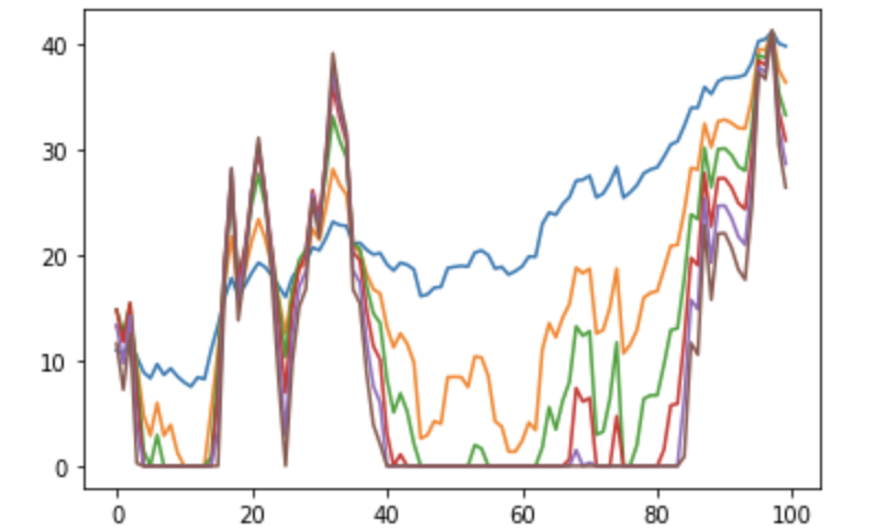
- Use some data that we generated for this purpose that is “marketing-spend-like” in that it is strictly positive and highly correlated. It looks like this (and you can download it at this link).
- Generate a “sales” variable according to a formula so that we know the true relationship between the spend variable and sales
- Run an OLS regression and observe the negative coefficients
- Run our OLS model using the Bayesian framework and observe that we get the same results
- Adjust our Bayesian OLS model so that the coefficients must be positive and see how our results improve
OLS
First thing we’ll need to do is generate our dependent variable. I generated the variable like this:
sales = (20 + spend_data['channel_1'] * 1.1 + spend_data['channel_2'] * 0.7 +
         spend_data['channel_3'] * 0.8 + spend_data['channel_4'] *1.5 +
         spend_data['channel_5'] * 0.8 + spend_data['channel_6'] * 0.95 +
         np.random.normal(20, 5, size=len(spend_data['channel_1']))
  )
So we can see that we have an intercept of 20 and the following schedule of true coefficients:
| Variable | True ROI |
|---|---|
| Intercept | 20 |
| Channel 1 | 1.1 |
| Channel 2 | 0.7 |
| Channel 3 | 0.8 |
| Channel 4 | 1.5 |
| Channel 5 | 0.8 |
| Channel 6 | 0.95 |
The results of our OLS model look like this:
est = sm.OLS(sales, spend_data_with_c).fit()
est.summary()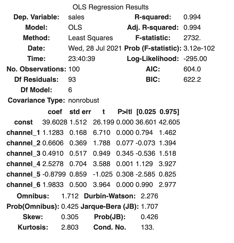
We can see that our results are highly biased, meaning the estimate doesn’t match what we know to be the true ROI. Note also that we have a very high R-squared of 0.994, even though we know that these results are very wrong. R-squared definitely isn’t everything!
| Variable | True ROI | OLS Estimate |
|---|---|---|
| Intercept | 20 | 39.6 |
| Channel 1 | 1.1 | 1.1 |
| Channel 2 | 0.7 | 0.7 |
| Channel 3 | 0.8 | 0.5 |
| Channel 4 | 1.5 | 2.5 |
| Channel 5 | 0.8 | -0.9 |
| Channel 6 | 0.95 | 2.0 |
Channels 4,5, and 6, in particular, are way off. Channel 5 is getting a negative effect!
Introducing Bayesian Framework with PyMC3
Just to prove to ourselves that we know what we’re doing, let’s run the exact same model using the PyMC3 framework.
with pm.Model() as model:
    sigma = pm.HalfNormal("sigma", sd=1) # This is our error term
    intercept = pm.Normal("Intercept", 0, sigma=20) # Our intercept
    beta = pm.Normal("x", 0, sigma=20, shape = 6) # These are our betas
    # And here is our regression formula!
    mu = intercept + beta[0] * spend_data['channel_1'] + beta[1] * spend_data['channel_2'] + beta[2] * spend_data['channel_3'] + beta[3] * spend_data['channel_4'] + beta[4] * spend_data['channel_5'] + beta[5] * spend_data['channel_6']

    # Here is where we fit our predictions (mu) to the sales (observed)
    Y_obs = pm.Normal("Y_obs", mu=mu, sigma=sigma, observed=sales)

    # Here’s where we run the MCMC simulation
    ols_trace = pm.sample(2000, cores=2)
While this probably looks pretty intimidating if you’re not familiar with Bayesian modeling, what this code block is doing is just laying out each of the assumptions of the OLS regression individually. We won’t get into the weeds now, but we can be sure that we did it correctly because we generate the same results we got with our original “traditional” OLS.
| Mean | |
|---|---|
| Intercept | 39.422422 |
| beta_1 | 1.141292 |
| beta_2 | 0.646379 |
| beta_3 | 0.503570 |
| beta_4 | 2.509949 |
| beta_5 | -0.852193 |
| beta_6 | 1.968111 |
| sigma | 4.408570 |
Here we can see our estimate for the intercept and each of our 6 beta coefficients. So here’s our summary of what we’ve seen so far. Bayesian OLS gives the same results as traditional OLS, still very problematically biased.
| Variable | True ROI | OLS Estimate | Bayesian OLS |
|---|---|---|---|
| Intercept | 20 | 39.6 | 39.4 |
| Channel 1 | 1.1 | 1.1 | 1.1 |
| Channel 2 | 0.7 | 0.7 | 0.7 |
| Channel 3 | 0.8 | 0.5 | 0.5 |
| Channel 4 | 1.5 | 2.5 | 2.5 |
| Channel 5 | 0.8 | -0.9 | -0.9 |
| Channel 6 | 0.95 | 2.0 | 2.0 |
Improving Bayesian OLS
So finally we want to tweak our OLS assumptions to better match our beliefs about marketing spend — namely, that coefficients can’t be negative. Let’s see how that looks in code:
with pm.Model() as model:
    sigma = pm.HalfNormal("sigma", sd=1)
    intercept = pm.Normal("Intercept", 0, sigma=20)
    # This Section is Changed!
    #####################
    BoundedNormal = pm.Bound(pm.Normal, lower=0.0)
    beta = BoundedNormal("x", 0, sigma=20, shape = 6)
    #####################
    mu = intercept + beta[0] * spend_data['channel_1'] + beta[1] * spend_data['channel_2'] + beta[2] * spend_data['channel_3'] + beta[3] * spend_data['channel_4'] + beta[4] * spend_data['channel_5'] + beta[5] * spend_data['channel_6']

    Y_obs = pm.Normal("Y_obs", mu=mu, sigma=sigma, observed=sales)
I’ve highlighted the only two lines that we changed in the model. While the syntax is dense, all that we’ve done is taken our assumption about the beta coefficient and changed it from a normal distribution to a normal distribution that’s bounded at 0.
Once we run this model, we get the following results:
| Mean | |
|---|---|
| Intercept | 39.2522177 |
| beta_1 | 4.434134 |
| beta_2 | 1.161251 |
| beta_3 | 0.588905 |
| beta_4 | 0.720421 |
| beta_5 | 1.773296 |
| beta_6 | 0.294285 |
| sigma | 1.378123 |
Which we can use to update our summary table
| Variable | True ROI | OLS Estimate | Bayesian | Bounded Bayesian |
|---|---|---|---|---|
| Intercept | 20 | 39.6 | 39.4 | 39.3 |
| Channel 1 | 1.1 | 1.1 | 1.1 | 1.2 |
| Channel 2 | 0.7 | 0.7 | 0.7 | 0.6 |
| Channel 3 | 0.8 | 0.5 | 0.5 | 0.8 |
| Channel 4 | 1.5 | 2.5 | 2.5 | 1.7 |
| Channel 5 | 0.8 | -0.9 | -0.9 | 0.3 |
| Channel 6 | 0.95 | 2.0 | 2.0 | 1.4 |
Still biased! But much closer to our true estimates, and with no totally nonsensical negative-impact results.
Conclusion
While this is a big step forward for our model, it definitely doesn’t solve all of our problems. Our results here are still biased and could lead us to make the wrong decisions for our marketing program. And this was a very simplified example — we haven’t even started dealing with other features of marketing spend that are critical to handle to build a realistic model. Things like:
- Channel saturation and declining marginal efficiency of spend
- Time shifts between when dollars are spent and when the effect is realized
- “Organic” conversions
- Seasonality
All of these features are critical to include in any MMM model that you’re going to use to make decisions about your marketing spend.
At Recast, we handle all this for you, having spent years working with the world’s top marketers to correctly model the way marketing works in the real world. The flexibility of Bayesian techniques is what lets us do all of this automatically in real time – if you’ve set sensible priors, there’s just less need for human intervention to correct for ‘unrealistic’ coefficients! Give us a shout if you’d like to learn more.