
Monte Carlo simulations are a powerful tool for doing predictive analysis. By running multiple simulations with different input variables, analysts can gain insight into the likelihood of different outcomes and make more informed decisions. In this blog post, we’ll explore what Monte Carlo simulations are, how they work, and run through some examples of their practical applications, including code in Python and R. We will also discuss the use of Monte Carlo simulations in Bayesian MCMC Marketing Mix Modeling, a modern technique for analyzing marketing data and allocating marketing budgets through proper attribution. Whether you’re new to Monte Carlo simulations or just looking to deepen your understanding, this post should have you covered.
I. Introduction to Monte Carlo simulations
- Definition and explanation of Monte Carlo simulations
- Examples of practical applications
II. How Monte Carlo simulations work
- Overview of the process and key components
- Discussion of random sampling and statistical analysis
III. Monte Carlo simulations in Bayesian MCMC Marketing Mix Modeling
- Explanation of marketing mix modeling and its importance
- Discussion of how Monte Carlo simulations can be used in this context
IV. Code examples in Python and R
- Simple examples of Monte Carlo simulations in both languages
- Discussion of how these examples can be expanded and adapted for more complex applications
V. Conclusion
- Recap of key points and takeaways
- Encouragement to learn more and explore the benefits of Monte Carlo simulations for yourself.
I. Introduction to Monte Carlo simulations
Monte Carlo simulations are a statistical method for understanding and predicting complex systems under conditions of uncertainty. They were developed by mathematician Stanislaw Ulam and physicist John von Neumann (of Manhattan Project fame) in the 1940,. The method gets its name from Monte Carlo, a city in Monaco known for its casinos, because the simulations rely on the element of chance, using random sampling to generate results. By running multiple simulations with different input variables, analysts can gain insight into the likelihood of different outcomes and make more informed decisions, much like playing thousands of games of roulette and counting the times you win, to work out the odds.
Monte Carlo simulations are used in a variety of fields, including finance, engineering, and meteorology, as well as marketing. In finance, for example, Monte Carlo simulations can be used to model the performance of investment portfolios and predict the likelihood of different returns. In engineering, Monte Carlo simulations can be used to understand the behavior of complex systems, such as the airflow around an aircraft wing. In meteorology, Monte Carlo simulations can be used to predict the likelihood of different weather patterns and their impacts. In marketing, Monte Carlo simulations can be used in Bayesian MCMC Marketing Mix Modeling to analyze data and allocate marketing budgets through proper attribution. These are just a few examples of the many practical applications of Monte Carlo simulations, though it has by now impacted most fields of study.
One of the key benefits of Monte Carlo simulations is their ability to provide a probabilistic view of a system, rather than a single point estimate. By generating a distribution of potential outcomes, Monte Carlo simulations allow analysts to understand the full range of possible outcomes and their likelihoods, rather than just a single “best guess” prediction. This surfaces the inherent uncertainty in decision-making, keeping the decision maker more informed about the odds. This can be particularly useful in situations where the input variables are uncertain or there is a high degree of variability in the system.
However, Monte Carlo simulations are not without their limitations. One of the biggest challenges is developing an accurate and realistic mathematical model of the system. This requires a deep domain expertise and the underlying dynamics of the system, as well as access to reliable data and some knowledge of statistics. Another challenge is the computational cost of running multiple simulations, which can be time-consuming and require significant computing power. Finally, the results of Monte Carlo simulations are only as good as the input assumptions and the underlying model, so analysts must be careful to validate their assumptions and verify the accuracy of the results.
In recent years, Monte Carlo simulations have come into greater use due to several factors. One is the availability of more powerful computers and advanced algorithms, which make it possible to run larger and more complex simulations in a reasonable amount of time. Another is the proliferation of data, which has increased the amount of information available to inform the input assumptions and validate the results of Monte Carlo simulations. Finally, the increasing complexity of modern systems, including global financial markets and large-scale engineering projects, has made Monte Carlo simulations an increasingly valuable tool for analyzing and predicting their behavior. Together, these factors have contributed to the growing popularity and importance of Monte Carlo simulations in a variety of fields, including Marketing.
II. How Monte Carlo simulations work
Monte Carlo simulations are a powerful tool for understanding and predicting complex systems, but how do they actually work? At a high level, the process involves the following steps:
- Identify the system you want to analyze and the input variables that affect its behavior.
- Develop a mathematical model of the system that describes how the input variables impact the output.
- Define a range of possible values for each input variable, known as priors, based on available data and expert knowledge.
- Use random sampling to generate a large number of input combinations, each representing a potential realistic scenario for the system.
- Use the mathematical model to calculate the output for each scenario, resulting in a distribution of potential outcomes.
- Use statistical analysis to interpret the results and gain insights into the likelihood of different outcomes.
These steps can be repeated with different sets of input variables and ranges to explore a variety of scenarios and gain a more complete understanding of the system. Additionally, Monte Carlo simulations can be enhanced with more advanced techniques, such as optimization algorithms (finding the best possible combination of inputs to maximize output) and sensitivity analysis (identifying how much leverage each variable has over the outcome), to further complement the predictions.
Monte Carlo Simulation Example
Imagine you’re playing a game where you toss a coin and if it lands on heads, you win a prize. You can toss the coin as many times as you want, but you only get one prize at the end. The more times you toss the coin, the better your chances of winning will be. However the person who invited you to play this game is untrustworthy: they have a history of cheating! You can’t be sure if they’re using a real coin, where the odds are 50:50 between heads and tails, or a trick coin, which is weighted to land more on one side than the other.
You could toss the coin thousands of times to tell if the game was rigged, but that would be slow and tiresome. Instead you can have a computer program simulate tossing the coin many times to see how often it lands on heads. This would give you an idea of your chances of winning the game if you play it many times: is it a fair coin, or weighted on one side? This is what’s called a Monte Carlo simulation.
For example, if the program simulates tossing the coin 100 times and it lands on heads 60 times, then your chances of winning the game are about 60%. The more times the program simulates tossing the coin, the more accurate the simulation will be. If it lands on heads 600 times out of 1,000, you can be more certain the true chances of winning the game are 60%, than if you just simulated 100 flips.
So, a Monte Carlo simulation is like a way of predicting what will happen in a game, or real life scenario, by having a computer simulate it many times and see what happens on average. It’s a useful tool for understanding complex systems and making predictions.
Monte Carlo Simulation Formula
There is no specific formula for Monte Carlo simulation: as a technique it can be used to simulate the outcomes for any mathematical formula. Nor does the Monte Carlo technique need to be Bayesian, however these techniques are commonly paired together. One form that’s in popular use in Marketing is Bayesian Monte Carlo, also known as Markov Chain Monte Carlo (MCMC). This method is highly efficient and optimized for exploring a vast expanse of potential outcomes.
The general form of the formula for Bayesian Monte Carlo is:
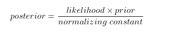
This formula can be used to approximate the posterior distribution of a given problem using random samples using Bayesian Monte Carlo methods. Here, the “posterior” is the distribution of the variables you are trying to estimate, the “likelihood” is the probability of the data given the model, the “prior” is the probability of the variables before observing the data, and the “normalizing constant” is a scaling factor that ensures the posterior is a valid probability distribution.
To apply Bayesian Monte Carlo, you first need to specify a model for the data and define the prior distribution of the variables you want to estimate. Then, you use random sampling to generate samples from the prior distribution and use these samples as input to the model. The outputs of the model are then used to calculate the likelihood of the data given the model.
Finally, the posterior distribution is approximated by combining the prior distribution and the likelihood using the formula above. This allows you to estimate the values of the variables and their uncertainty.
The exact form of the formula for Bayesian Monte Carlo will depend on the specifics of the problem you are trying to solve and the model you are using. In general, however, the formula involves combining probabilities and using random sampling to approximate the posterior distribution.
Random Sampling and Statistical Analysis
Random sampling is key to Monte Carlo methods, as it is used to generate samples from the prior distribution of the variables you want to estimate. This involves using probability distributions or other methods to determine the likelihood of each value, and then generating random samples that reflect these probabilities. For example, if you are trying to estimate the mean and standard deviation of a population, you might use a normal distribution as the prior and generate random samples of the mean and standard deviation from this distribution.
Once you have generated the random samples, you can use them as input to your model and run the simulation many times to generate a range of possible outcomes. This is known as running the Markov Chain, and it is an important step in Bayesian Monte Carlo because it allows you to generate a large number of samples from the posterior distribution.
After running the Markov Chain, you can use statistical analysis to analyze the results of the simulations and generate predictions or estimates for the problem you are trying to solve. This typically involves calculating summary statistics, such as the mean and standard deviation, and using these to make inferences – estimations of what effect inputs have on outputs of the model – about the posterior distribution.
Random sampling and statistical analysis are essential components of Bayesian Monte Carlo, and they are used together to generate predictions or estimates for a given problem using random samples from the prior distribution.
III. Monte Carlo simulations in Bayesian MCMC Marketing Mix Modeling
Marketing mix modeling is a statistical technique that is used to understand the effectiveness of marketing campaigns and to optimize marketing spend. It involves using data from various sources, such as sales, marketing spend, and consumer behavior, to build a model of the relationship between marketing variables and business outcomes. Marketing mix modeling is important because it allows businesses to make data-driven decisions about their marketing strategy, without the need for user-level data. This makes it robust to loss of tracking data due to privacy legislation or restrictions on collection of personally identifiable information. By understanding how different marketing activities affect sales, companies can optimize their marketing spend and improve the ROI of their campaigns.
Monte Carlo simulations can be used in the context of marketing mix modeling to generate a range of possible outcomes for different marketing scenarios. For example, a Monte Carlo simulation might be used to generate a range of possible sales figures for a product, given different levels of marketing spend. This can help businesses understand the potential impact of different marketing strategies and make more informed decisions about their marketing mix.
Additionally, Monte Carlo simulations can be used in Bayesian MCMC marketing mix modeling to incorporate uncertainty and probabilistic reasoning into the modeling process. This can provide a more realistic representation of the underlying system and allow for more accurate predictions or estimates, as well as providing flexibility in incorporating domain expertise into the construction of the model.
In Bayesian MCMC, the goal is to estimate the posterior distribution of a given problem using random samples from the prior distribution. This is done by specifying a model for the data and defining the prior distribution of the variables you want to estimate. Then, random sampling is used to generate samples from the prior distribution, and these samples are used as input to the model. The outputs of the model are then used to calculate the likelihood of the data given the model, and the posterior distribution is approximated by combining the prior distribution and the likelihood using a mathematical formula. This allows you to estimate the values of the variables and their uncertainty.
One of the key advantages of Bayesian MCMC is that it allows you to incorporate uncertainty and probabilistic reasoning into the modeling process. This is important because real-world systems are often complex and uncertain, and traditional statistical methods may not be able to accurately capture this complexity. Bayesian MCMC provides a more flexible and realistic approach to modeling, which can lead to more accurate predictions or estimates.
Additionally, Bayesian MCMC allows you to incorporate prior information or expert knowledge into the modeling process, through the use of Bayesian priors. This can be useful when there is existing information about the problem you are trying to solve, such as historical data or expert opinions, or where traditional statistical models regularly produce implausible results. By incorporating this information into the prior distribution, you can improve the accuracy and plausibility of the posterior estimates.
Overall, Monte Carlo simulations are a powerful tool for marketing mix modeling, and they can be used to generate a range of possible outcomes and incorporate uncertainty into the modeling process. This can help businesses make more informed decisions about their marketing strategy and optimize their marketing spend.
IV. Code examples in Python and R
In this section, we will look at code examples of Monte Carlo simulations in Python and R. These examples will show how to generate random samples from a probability distribution and use these samples to approximate a posterior distribution.This is a simple Monte Carlo simulation that can be used to understand the distribution of a given variable.
We will then discuss how these examples can be expanded and adapted for more complex applications. For instance, you could use Monte Carlo simulation to estimate the posterior distribution of a marketing mix model and generate predictions for different marketing scenarios.
These code examples will provide a starting point for understanding Monte Carlo simulation in Python and R, and they can be adapted and expanded for a wide range of applications.
Here are some simple examples of Monte Carlo simulations in Python and R:
Python:
# Import the necessary libraries
import numpy as np
import matplotlib.pyplot as plt
# Define the number of simulations
n_simulations = 1000
# Generate random samples from a normal distribution
samples = np.random.normal(0, 1, n_simulations)
# Plot the histogram of the samples
plt.hist(samples)
plt.show()
R:
# Load the necessary libraries
library(tidyverse)
library(ggplot2)
# Set the number of simulations
n_simulations <- 1000
# Generate random samples from a normal distribution
samples <- rnorm(n_simulations, 0, 1)
# Plot the histogram of the samples
ggplot(data.frame(samples), aes(x = samples)) +
geom_histogram(bins = 50)
These examples show how to generate random samples from a normal distribution and plot the histogram of the samples. This is a simple Monte Carlo simulation that can be used to understand the distribution of a given variable.
These examples can be expanded and adapted for more complex applications by incorporating more variables, using more advanced models, and incorporating additional analysis steps. For example, you could use Monte Carlo simulation to estimate the posterior distribution of a marketing mix model and generate predictions for different marketing scenarios.
Here is an example of how you could accomplish this:
Python:
# Import the necessary libraries
import numpy as np
import pandas as pd
import seaborn as sns
# Load the data
data = pd.read_csv(“marketing_data.csv”)
# Define the number of simulations
n_simulations = 1000
# Generate random samples from the prior distribution
samples = np.random.multivariate_normal(mean=[0, 0, 0],
cov=[[1, 0, 0],
[0, 1, 0],
[0, 0, 1]],
size=n_simulations)
# Use the samples as input for the model and run the simulations
results = []
for i in range(n_simulations):
x1, x2, x3 = samples[i]
y = 2 * x1 + 3 * x2 + 4 * x3 + np.random.normal(0, 1)
results.append(y)
# Plot the histogram of the results
sns.histplot(results)
R:
# Load the necessary libraries
library(tidyverse)
library(MASS)
# Load the data
data <- read_csv(“marketing_data.csv”)
# Set the number of simulations
n_simulations <- 1000
# Generate random samples from the prior distribution
samples <- mvrnorm(n = n_simulations, mu = c(0, 0, 0), Sigma = diag(3))
# Use the samples as input for the model and run the simulations
results <- vector(“numeric”, length = n_simulations)
for (i in 1:n_simulations) {
x1 <- samples[i, 1]
x2 <- samples[i, 2]
x3 <- samples[i, 3]
y <- 2 * x1 + 3 * x2 + 4 * x3 + rnorm(1, 0, 1)
results[i] <- y
}
# Plot the histogram of the results
ggplot(data.frame(results), aes(x = results)) +
geom_histogram(bins = 50)
In this example, we start by loading the marketing data and defining the number of simulations. Then, we generate random samples from the prior distribution of the variables we want to estimate. In this case, we assume that the prior distribution is a multivariate normal distribution with a mean of [0, 0, 0] and a covariance matrix of [[1, 0, 0],[0, 1, 0], [0, 0, 1]].
Next, we use the samples as input to the model and run the simulations. In this example, we assume that the model is a linear regression with three predictors and one response variable. We use the samples to generate a range of possible values for the predictors, and we use these values as input to the model to generate a range of possible outcomes for the response variable.
Finally, we plot the histogram of the results to visualize the distribution of the possible outcomes. This allows us to see the range of possible values for the response variable, given the samples from the prior distribution.
Overall, this illustrative example shows how you could use Monte Carlo simulation to explore the range of outcomes assuming some range of possible input variables. It involves generating random samples from the prior distribution, using these samples as input to the model, and analyzing the results to generate predictions or estimates. In practice models will be more complex, and built custom for the specific problem you are trying to model, by a data scientist with experience in this domain.
V. Conclusion
In conclusion, Monte Carlo simulations are a widely-used method for predictive analysis and decision making. By simulating multiple scenarios with different input variables, analysts can gain insight into the likelihood of different outcomes and make more informed decisions, with respect to uncertain conditions. This blog post discussed the basics of Monte Carlo simulations, how they work, and some examples of their practical applications. We also discussed the use of Monte Carlo simulations in Bayesian MCMC Marketing Mix Modeling, a technique for analyzing marketing data and allocating marketing budgets. We hope that this post has provided useful information and insights, whether you are new to Monte Carlo simulations or looking to deepen your understanding of the topic.