
Disclaimer: This blog post was written by an external contributor about detecting and addressing heteroskedasticity in marketing mix models. The approach laid out in this document is not reflective of how Recast approaches heteroskedasticity and model validation. The actual model specification can be found in the technical model specification.
Heteroskedasticity in a regression model is when the variance of the residuals varies with each observation. Most statistical software assumes that the errors made in prediction are random noise, or in statistics speak, the variance of the residuals is constant for all observations, which is called homoskedasticity. Heteroskedasticity, where there’s a pattern in the errors is a serious problem that needs to be addressed directly or else the conclusions from your model may be invalid.
We draw conclusions about how we should allocate our marketing spend by interpreting the coefficients of our Marketing Mix Model. The coefficients tell us how spend on each marketing channel affects sales. We can also use statistical tests to determine if a particular channel, or group of channels, has any significant impact on sales. For example, we might estimate a positive coefficient for spend on Display advertising, but the coefficient might not be significantly different from zero. The t-test and F-test are two well-known statistical tests that we can use, that are common in traditional econometrics (though this isn’t the only way, for example Recast validate their model using modern testing methods).
When we have heteroskedastic errors, the coefficients will still be unbiased. But the standard errors will be incorrect. The variance estimates will be misleading. And the results of t-tests and F-tests will be invalid. How can we fix the heteroskedasticity problem and perform residual tests in our Marketing Mix Model?
Our Marketing Mix Modelling Scenario
In our scenario, we have an online store. We want to use a Marketing Mix Model to scientifically optimize our advertising spend. Our data analyst estimates the following regression equation.

sales at time t is the dependent variable. In our regression equation, sales is our y vector. Our spend on search, display, social, lagged sales, and a vector of all ones, make up the columns of the X matrix. et is the error at time t.
One of the assumptions of Ordinary Least Squares (OLS) regression is that the residuals have constant variance and are independent from each other. This assumption is known as homoscedasticity and non-autocorrelation.
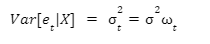
Homoskedastic errors are defined as:
Non-autocorrelation is defined as:
In summary, we define the assumption as:
Where e is the vector of regression residuals, X is the matrix input variables and I is the identity matrix. 2 is a scalar.
When all of the assumptions of OLS are satisfied, you can perform residual tests with standard software packages and their results will be valid.
Heteroskedastic errors are when Var(et| X) is not the same constant value for all t. When our regression has heteroskedastic errors, the standard errors will be incorrect. Hence, the estimates of the covariance of our coefficients will be incorrect. Although the coefficients will be unbiased, we will not be able to perform the standard t-tests and F-tests.
Detecting Heteroskedasticity
You can detect heteroskedasticity with residual plots and statistical tests. Visually exploring data is always a good idea. I recommend creating residual plots even if you intend to rely mostly on the results of statistical tests. We’ll briefly explore methods for detecting heteroskedasticity before diving into techniques to fix it.
Residual Plots
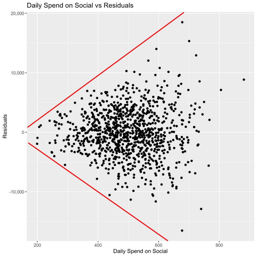
In the scatterplot above, we can see that the residuals from our regression “fan out” as our spend on social media advertising increases. I have drawn red lines to emphasize how the variance of the residuals increases as daily spend on social increases. This is a sign of heteroskedasticity. The variance of the residuals increases as spend on social media advertising increases.
Statistical Tests
The Goldfeld-Quant Test has a null hypothesis of homoscedasticity. The original 1965 Goldfeld-Quant paper proposed two tests, a parametric test and a nonparametric test. When someone doesn’t mention which Goldfeld-Quant test they are referring to, they usually mean the parametric test. The parametric version assumes that the errors follow a Normal distribution. OLS also assumes the errors follow a Normal distribution. The parametric version will do fine for our scenario.
The Breusch-Pagan/Godfrey Lagrange Multiplier Test also has a null hypothesis of homoscedasticity. It allows you to test if a particular set of variables is causing heteroskedasticity. It tests for the presence of heteroskedasticity in the form:
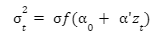
Where zt is a vector of independent variables. If the variables in zt are exactly the same as the variables in X, then this test is equivalent to another test for heteroskedasticity called White’s General Test.
Remedies for Heteroskedasticity
White’s Heteroskedasticity-Consistent (HC) Standard Errors
When our regression residuals are heteroskedastic, our coefficients are still unbiased. We can use White’s Heteroskedasticity-Consistent estimator to estimate the correct standard errors. With the correct standard errors, we can find confidence intervals for our parameters and perform t-tests.
If you are using R, then you can use the coeftest() and coefci() functions in the lmtest package. You will also need the vcovHC() function from the sandwich package. The coeftest() function calculates the t-test statistics and p-value. The coefci() function calculates the confidence intervals for the model parameters. The vcovHC() function estimates the heteroskedasticity-consistent covariance matrix. You need to pass the vcovHC() function to the coeftest() and coefci() functions by specifying “vcov.=vcovHC”, when calling those functions.
Weighted Least Squares
Weighted Least Squares assumes that we know the form of our heteroskedasticity. We either apply the weights to each observation and then run OLS. Or we can pass the weight vector to our statistical software. If you are using R, the lm() function has a “weights” parameter for passing the weight vector.
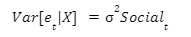
We assume that the covariance matrix has a certain form.
In our scenario, the heteroskedasticity is caused by our Social variable. We have multiple independent variables in our model, but only Social is causing heteroskedastic errors.
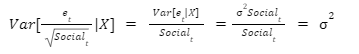
In order to weight each observation, we need to divide it by the square root of the non-constant component. In other words, our weight vector is:

We then fit the following regression.
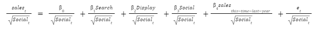
The weighted error term is constant for all observations.
Box-Cox Transformation
You can use transformations to normalize variables. Transformations work by squeezing more extreme values towards the less extreme. For example, imagine a variable that follows a Log-Normal distribution. If the σ parameter is high enough, then it would have a long tail to the right. When we apply the log transformation to this data, it becomes Normally distributed and well behaved.
There is a potential drawback of using transformations in a marketing mix model. For example, it is straightforward to interpret the meaning of a coefficient on a raw spend variable, which helps predict a raw sales variable. It is less straightforward to interpret a coefficient on a transformed spend variable, which helps predict a transformed sales variable.
The Box-Cox transformation is one of the most popular transformations. Taking the log is a special case of the Box-Cox transformation, where the Box-Cox parameter, 𝜆, equals zero. In order to apply the Box-Cox transformation, the variable that we are transforming must be positive. The variable cannot be zero or less. This might present a problem for companies where spend and sales are zero on some days.
The formula for the Box-Cox transformation is below. Note that you need to fit the parameter λ to your data. If you are using R, then you can use the BoxCox(), InvBoxCox() and BoxCox.lambda() functions in the forecast package. BoxCox.lambda() estimates the value of 𝜆 that best fits your data. BoxCox() applies the transformation, when given a value of 𝜆. InvBoxCox() inverts the transformation and gives you the un-transformed data.

Conclusion
As you can see, validating a marketing mix model can get particularly difficult rather quickly, and requires advanced statistical knowledge which you might not have on your team. If you haven’t encountered errors of this kind before you might not know the tricks for dealing with them, or may not even be aware that there’s a problem. That can leave you making conclusions the data doesn’t support, and allocating your budget to the wrong marketing channels, harming performance.