
Scenario planning or demand forecasting decides everything an enterprise does.
Right from quantities of raw material sourced to the inventory that needs to be stocked, through to shipping, packaging, hiring, and all the way down to purchasing office supplies — everything is dependent on accurate forecasting and scenario planning.
Forecasting errors can send ripples flowing down the entire chain as each link in the chain is dependent on the ones that precede and succeed it. It’s called the supply “chain” for a reason. A small stimulus at one end can amplify into a pulsating wave at the other end that can distort demand signals and make the most elaborately laid out business plans go haywire.
In marketing terms, this is called the bullwhip effect because of how forecasting errors on one end of the supply chain flow like waveforms that get amplified as they traverse upstream, much like how you would cause a bullwhip to ripple by jerking the wrist.

The bullwhip effect is a classic problem in demand forecasting.that is much researched but remains unresolved.
Mathematically, a very simple formula for expressing the bullwhip effect is
Variance of Order
Bullwhip Effect = ________________
Variance of Demand
A value greater than 1 implies orders exceed demand, a value of less than 1 implies demand exceeds orders, while a value of exactly 1 implies demand and order are in equilibrium.
While advanced time series forecasting techniques manage to reduce the bullwhip effect, errors persist.
For instance, consider a classic supply chain consisting of a retailer, wholesaler, and a manufacturer. The retailer may respond to a sudden demand spike by placing a larger order with the wholesaler. It calculates the quantum of this order by inputting demand signals into a time series-based forecasting model to arrive at a number. At this point, a small forecasting error is likely to creep in due to the inaccuracy of time series forecasting. To avoid being caught out of stock, the retailer may even order a little over this number as a buffer.
The wholesaler, anticipating even more future demand, would add their own forecast estimates to the numbers received from the retailer, and pass on an even further inflated order to the manufacturer.
And since the manufacturer produces at scale, it can not respond immediately to sudden demand spikes. To avoid this lag, it usually produces a slightly excess stock in each order cycle.
Receiving an already inflated order, it runs this number through its scenario planning models based on historical demand to arrive at its own demand forecast. At this point, the forecasting error has been compounded three times over.
The manufacturer then adds a little extra to this forecast as a buffer, resulting in a significantly larger production order. To meet this order, it may need to increase its workforce, deploy more logistics for transportation, and increase storage capacity.
Depending on the magnitude of the forecasting error, the manufacturer, who is located at the upper end of the supply chain experiencing the bullwhip effect, may end up with significant overproduction-related costs.
But why does scenario planning result in forecasting errors in the first place? To understand this, we first turn to understanding scenario planning models.
Understanding Scenario Planning Models
Scenario planning or demand forecasting is most commonly done using time series forecasting techniques. Historical sales data is used to predict future demand with the underlying assumption that given a large enough data set, patterns in historical time series data will replicate themselves in the future.
Time series forecasting techniques are broadly of four types:
- Traditional, that include techniques such as regression, exponential smoothing, and autoregressive integrated moving average (ARIMA)
- Machine learning based, which include artificial neural network forecasting, and Fuzzy Set Theory Based Neural Networks
- Bayesian Forecasting, including Bayesian Markov Chain Monte Carlo like is used at Recast. Facebook Prophet is Bayesian, as is Google’s LightweightMMM. uses probability distributions instead of point estimates, and works well with data that exhibits multiple seasonalities.
Irrespective of type, most scenario planning techniques use historical data, trends, and seasonality to forecast future demand. In doing so, they miss out on a critical input — the marketing mix and its effect on shaping demand.
So does introducing MMM to schedule planning lead to more accurate forecasting and reduced bullwhip effect?
A team of researchers led by Prof Ajay Kumar of the Harvard Business School decided to find out just that. They trained a fuzzy neural network (FNN) based time series model on demand and sales data for a TV manufacturing company. The data pertained to a period of 372 weeks between 2010 and 2017.
They then prepared another data set consisting of advertising spend by the manufacturer across different marketing channels such as television ads, mobile SMS, internet, and newspapers.
Both the data sets were used as the input for a FNN-based forecasting model.
The researchers found, unsurprisingly, that the bullwhip effect was almost 1. Which meant that the model was very good at predicting future demand and could be used in scenario planning and demand shaping.
Why Does Introducing MMM to Scenario Planning Yield Better Results?
Forecasting has three basic elements — demand sensing, demand shaping, and demand prediction. All three are sensitive to the effects of marketing.
Demand sensing is a measure of the fluctuations in demand over the short term. For instance, if we run an online ad today, and it results in increased demand over the next week, this is a demand sensing signal.
Demand shaping is when a business uses certain incentives such as price drops to influence demand. MMM makes demand shaping more precise. For instance, a price cut or a sale is quite pointless unless it is communicated to the customer through proper marketing channels.
Finally, demand prediction combines signals from demand sensing and demand shaping, which are then combined with historic time series data to arrive at a forecast. Since marketing is intimately tied with demand at every stage of this process, it becomes a crucial input for forecasting demand.
Scenario Planning in Excel Using Marketing Mix Modeling
We now turn to building a simple marketing mix model in Excel that will help us make sales forecasts.
To begin with, we’ll need data. We’ve used this dataset for the purpose of this post. It lists the weekly sales figures for a product, along with the ad spend for Facebook, TV, and radio ads. ( yes, we know no one listens to the radio anymore, but let’s pretend it’s still the summer of ‘69 and podcasts don’t yet exist)
We’ll use this historical data to predict future sales, and see how varying the composition of the marketing mix can impact future sales.

Next, we apply linear regression on this to create our model. This can be done using the LINEST function in Excel and Google Sheets.
This is what the syntax for the LINEST function looks like in Excel:

If we use Google Sheets, the syntax is the still the same though the nomenclature might look like this:

Here, known_data_y is the dependent variable whose value we wish to calculate. In this case, it is Sales.
Known_data_x is the independent variable or the input to the linear regression function. In this case, it is the ad spend numbers for FB, TV, and Radio ads.
Calculate_b is a constant value that determines the point at which the trend line of this data meets the Y-axis, also called the Y-intercept. It has its roots in the mathematical formula for linear regression:
Y = b1x1 + b2x2 + ….bnxn + a
Which in turn is derived from the mathematical general equation for any line
Y = ax + b
Where b is a constant that represents the Y-intercept, represented by Calculate_b in the LINEST function above.
Going back to our dataset, we select the appropriate values, enter them in the function, and hit enter. This gives us the following output:
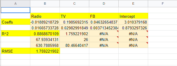
What this result gives us is four things:
- Coefficients
- R-squared or the model fit ( R^2) that measures how dependent variables vary relative to independent variables
- Root mean square error (RMSE) for each coefficient
- The intercept, which is the constant we discussed previously.
We are now going to use these coefficients to arrive at a sales prediction.
To do this, we use the linear regression formula we discussed earlier
Y = b1x1 + b2x2 + b3x3 + a
Where
- Y is the predicted sale value
- b1, b2, and b3 are the coefficients we just calculated above
- x1, x2, and x3 are the values for FB, TV, and Radio ad spend we see in our dataset.
- And a is the intercept.
To see our predictions, we copy the sales data in one column, and to the next column apply the formula discussed above. This is what the result would look like:
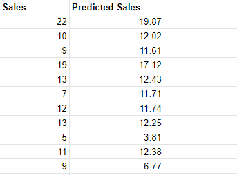
So we’ve now created a very simple forecast. We call this simple because we have not taken into account the effect of adstock and diminishing returns on ad spend.
Adstock measures the impact of an advertisement over time. Diminishing return measures how a marketing channel gets saturated over time to the point where increased investments do not translate into increased sales. Adding these two parameters to the model will increase its accuracy and its relevance, because in any real world scenario, adstock and diminishing returns are significant, and almost inevitable phenomena.
For the sake of simplicity however, we will skip this for now and move on to the next step, which is scenario optimization.
Scenario Optimization Using Solver
We’ve used MMM to create a simple forecast that takes into account historical sales data in conjunction with our marketing spend on various channels. What we’re interested in next is finding out how we should allocate our marketing budget to each of our marketing channels to maximize this predicted sales value.
Here’s how we can do it in Excel.
Step 1: Activate Solver in Excel
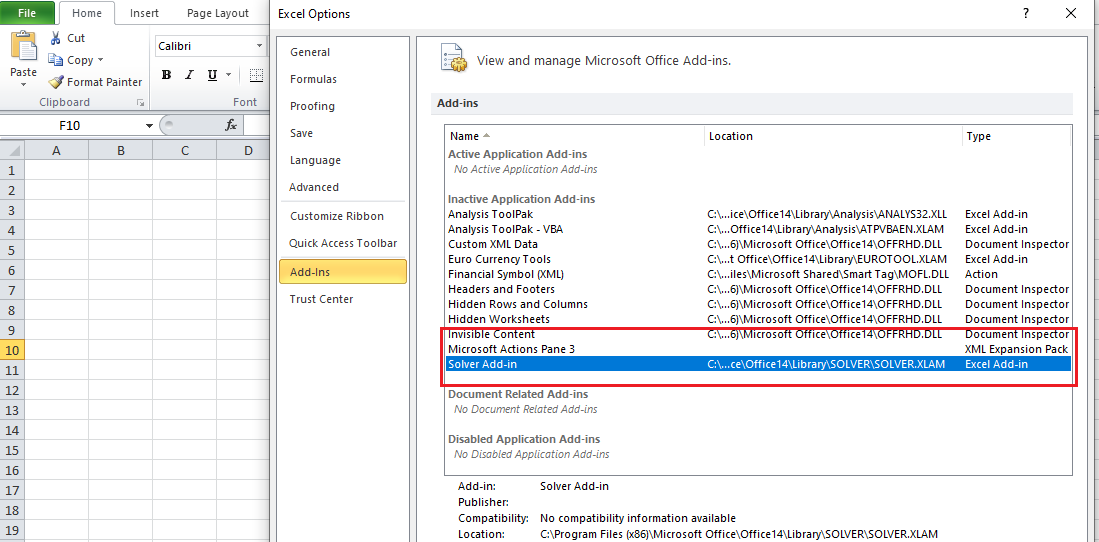
Solver comes as an add-in in Excel, and if you’ve never used Solver before, you will need to activate it. To do this, click on the File menu, then Options, and then Add-ins.
This opens up a dialog box like the one shown below. Click on Solver Add-in, followed by Go, and then OK.
Once Solver is added, it will show up under the Data tab on the far right of the top menu like this:

Step 2: Load Your Data
Next, we populate our excel sheet with the data we’re looking to optimize. While doing so, we add an extra [parameter this time — Maximum Budget.
This defines the maximum marketing budget we have at our disposal. Solver will show us the most optimal marketing mix based on this value. If we don’t enter this constraint, there is no limit to what the maximum amount we can spend on each marketing channel, and thus the optimal value would tend to be as high as is numerically possible.
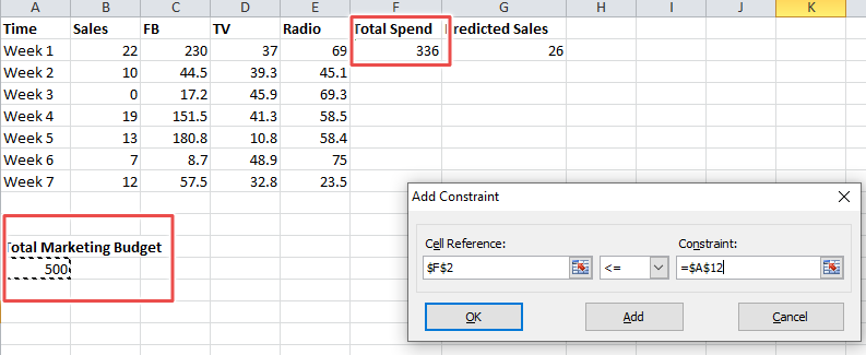
For convenience’s sake, we’ve set the total marketing budget value to 500. We’ve also added a new column Total Spend which is the sum of the marketing spend across the three channels, and which must be kept below the total marketing budget.

Step 3: Launch Solver
Click on the Solver icon on the panel. This opens up a dialog box in which we are required to fill in the parameters for Solver to optimize.
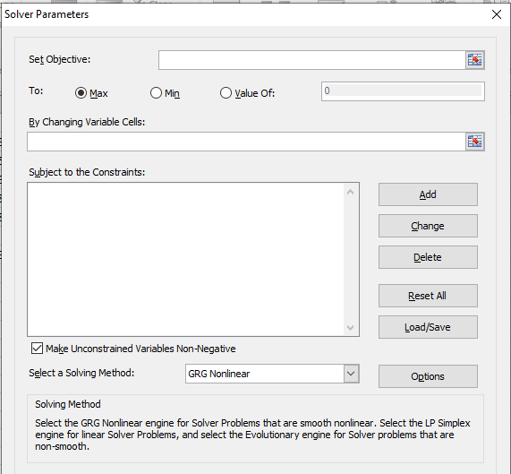
Step 4: Enter Parameters
The first parameter we are required to fill in is Set Objective.
Since our objective is to maximize sales, we select the value(s) in the Predicted Sales column, then select the Max radio button below it.

The next thing we need to select are the variables that Solver would optimize to achieve this result. In our case, these variables are the marketing spend values for each of the three channels.
When we select the three values, they show up in the box labeled By Changing Variable Cells.
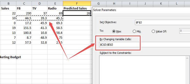
Thus far, we’ve told Solver that we want to maximize sales by changing the values of three variables.
So far so good.
The next thing it needs to know is if there are any constraints involved. The answer to this, as we just discussed, is yes. Our marketing budget is the constraint.
We click on Add Constraint and specify that the total spend should be less than the marketing budget.
We click on OK and then hit Solve.
Solver then presents to us the most optimal marketing mix allocation which would maximize our predicted sales under the given conditions.
And that’s it. We’ve built a simple scenario planning model using MMM and optimized it for maximum sales. All using the humble Excel.
It bears repeating once again that this is a very simple model. We could add several layers of complexity to make it more accurate and more powerful so that it becomes capable of delivering forecasts even when working with data the model hasn’t seen. For instance, we could implement neural networks within this Excel model, or execute it using R, or combine the two to have a neural network based forecasting model with MMM in R, and so on.
To Sum Up
We’ve seen in this post the theory behind why traditional time series forecasting techniques are prone to the bullwhip effect, and why including MMM into forecasting helps reduce forecasting error.
We’ve also seen how to build a simple marketing mix model, use it for forecasting future sales, and then use Excel Solver for optimizing our marketing spend to maximize sales.
We can add more complexity, and more accuracy to this model by using a neural network in place of simple regression analysis. We could also use Python to build a marketing mix model instead of Excel, or by including the effects of adstock and diminishing returns. The point however, was to demonstrate how MMM is a critical but often overlooked component of scenario planning and demand forecasting, and how businesses can benefit by including it in their scenario planning models.


