Linear regression is one of the most well known and well understood algorithms in statistics and machine learning. Anybody with access to Excel or Google Sheets can use linear regression, but don’t let its simplicity and accessibility fool you – it’s unreasonably effective at solving a long list of common problems, making it the workhorse of the marketing analytics world.
In this post you’ll see an example of a simple linear regression model, and learn how it works so you know how best to use it to find insights from your marketing data. In this post you will learn:
- What a simple linear regression model looks like in Excel / Google Sheets
- The benefits of adding more variables with multiple linear regression
- What the difference is between logistic and linear regression
- Whether linear regression counts as machine learning or if it’s just plain statistics
- What the linear regression equation is, and what assumptions we’re making in using it
- How to use a linear regression calculator in Excel / Google Sheets (+ free template)
- When it makes sense to use Python’s SKLearn library instead (+ free script)
You do not need to know a lot about statistics or mathematics to use linear regression. This is a beginner-level introduction to the technique to give you enough background to be able to use it to solve business problems, and understand how best to interpret the findings from data science projects you delegate to your team.
Having been around for more than 200 years, and has been studied from every possible angle. Unfortunately that makes learning about linear regression confusing for a beginner, because a lot of prior knowledge is often assumed, and multiple names are used interchangeably.
Simple Linear Regression Model
In its most basic sense, linear regression is a statistical model that assumes a linear relationship between the input variables (x) and a single output variable (y). Specifically it assumes that y can be calculated from a linear combination of the input variables. For example the amount you spend on advertising (x) affects the number of sales you get (y). Once we have the model, we can estimate how many sales you’ll get for each dollar spent on ads.
Linear Regression Formula
The formula for simple linear regression with one x variable looks like this:
y = B1*x + B0
Where
- y is the number of sales
- B1 is the coefficient for advertising, i.e. how many sales you get for each dollar spent
- x is how many dollars you spend on advertising
- B0 is how many sales you’d get if you spent $0 on ads
When a coefficient becomes zero, it effectively removes the influence of that variable on the model. If you spend zero dollars on advertising one month, the model would predict the baseline average sales, or the intercept, represented in the formula by B0.
Linear Regression Calculator in Excel / Google Sheets
If you’ve ever fit a trendline in Excel or Google Sheets, congratulations you’ve done simple linear regression! Display the equation on the chart and you get the values for the coefficient (B1), and the intercept or constant (B0). This is by far the simplest way to run a linear regression so I suggest you try it out now to see how easy it is, if you haven’t already.
To make it easy to understand, we’ve built a linear regression calculator in Google Sheets that you can also download as an Excel file. It comes ready with example data, but you can paste over it with your own to update the chart in the template.
- Visit this link to get some example data (if you don’t have your own)
- Select all the data in the two columns containing your x and y variable
- Click Insert > Chart > Scatter chart. Your y variable should be on the vertical axis
- Add a trendline > Show R2 > Show equation to display the formula
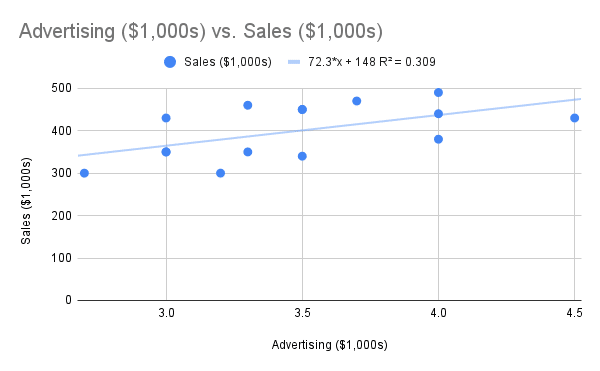
This is the same regression equation we saw in the previous section, with the model estimating that we get $72.3 in sales per dollar spent on advertising (both axes are in thousands). The intercept or constant, i.e. the baseline sales we would get without any advertising, is estimated at $148,000.
If we want to calculate how many sales we would get per week for a $2,000 weekly advertising budget, we could plug the numbers into the equation to get our prediction from the model.
72.3 * 2 + 148 = 292.6 thousand dollars
The R2 value of 0.302 tells us this model can explain 30.2% of the sales data knowing only the amount spent on advertising, a relatively weak correlation. Of course we can’t fully explain the number of sales we’ll get with this one variable – sales are affected by many different factors like the price of the product or if there’s a holiday. However this simple model is better than random guessing, and it took very little time or effort to build.
Multiple Linear Regression
When there is a single input variable (x), the method is referred to as simple linear regression. When there are multiple input variables, statisticians refer to the method as multiple linear regression.
We mentioned in the previous section that a simple model with just one variable representing the amount spent on advertising doesn’t take into account all the factors that drive sales. If we add additional x variables we can start to account for these other factors and improve the accuracy of our model.
For multiple variables we can no longer rely on our chart trendline, as each new variable represents another dimension. We can handle 3D charts but any more variables than that can’t easily be interpreted visually. We now need to move to using the LINEST function offered by both Excel and Google Sheets. The LINEST function works as follows:
LINEST(known_y’s, [known_x’s], [const], [stats])
Where
- known_y’s is the y variable we’re trying to predict
- known_x’s are the multiple x columns we’re using as inputs to our model
- const is whether we want to include the intercept or baseline in our model
- stats is how descriptive we want the output of the function to be
Pro Tip: when you use the LINEST function, the results come out backwards! The very first cell in the first row is the coefficient for the last variable you imputed, and they continue in reverse order from there. The final number in the top row is the coefficient for the intercept or constant.
- Visit this link to get access to the template and example data
- Use the LINEST function, inputting your y column and multiple x columns
- Put a 1 for the const and stats parameters
- The output of the first row are your coefficients
- The first number on the left in the third row is your model’s R2 value
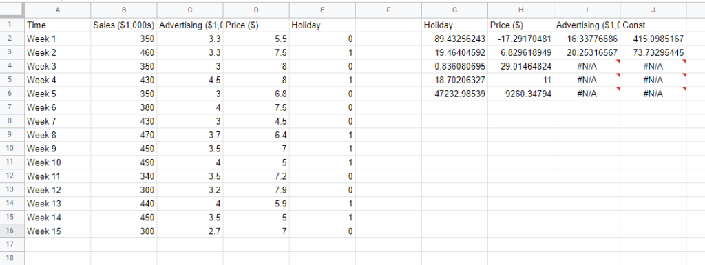
In our example we can see that our model is far better at explaining the data, with an R2 value of 0.83. We also get a radically updated coefficient for advertising. In our simple linear regression it was estimated as 72.3 dollars in sales per one dollar spent on advertising, and now we have a more realistic coefficient of $16. The Price coefficient can be interpreted as for every $1 increase in the price of the product, we lose $17,000 in sales. For Holiday the coefficient means we make $89,000 more on holidays than not holidays. Finally the constant or intercept says we make $415,000 in sales on average per week when Advertising, Price, and Holiday are accounted for.
Linear Regression Equation
To work out the predicted sales from our multiple regression model is a little more complicated than simple linear regression, but it’s the same basic formula. We have the y variable which is sales, and B0 which is the constant or intercept, but this time we have multiple x variables. Each x variable is multiplied by a corresponding B1, B2, B3 variable, which represents the coefficient, then those values are added together at the end.
y = B3*x3 + B2*x2 + B1*x1 + B0
Where
- y is the number of sales
- B3 is the coefficient for holiday, i.e. how many sales you get when it’s a holiday
- B2 is the coefficient for price, i.e. how many sales you lose for increases in price
- B1 is the coefficient for advertising, i.e. how many sales you get for each dollar spent
- x3 is whether it’s a holiday or not
- x2 is the price of the product
- x1 is how many dollars you spend on advertising
- B0 is how many sales you’d get if you spent $0 on ads
If we want to make a prediction with this multiple linear regression model we just plug in the coefficients as we did before, and find the y value.
89 * 0 + -17 * 6.6 + 16 * 2 + 415 = 334.8 thousand dollars
We know from the coefficients that holidays are worth $89,000 in extra sales and each $1 increase in price loses $17,000 in sales, but we need to input hypothetical future values to make this forecast. If we enter zero for holiday, that term multiplies to zero, so that variable won’t have an impact. For price let’s use the average which was $6.6. Finally let’s assume we spend $2,000 in ad spend. We also must remember to add the baseline sales from the constant which was $415,000.
Ordinary Least Squares (OLS)
How does Excel or Google Sheets actually build your linear regression model? It uses Ordinary Least Squares (OLS), the most popular method for building a linear regression model. It in effect draws a line of best fit between the points of data you have, minimizing the difference between where the line runs and the point on the chart.
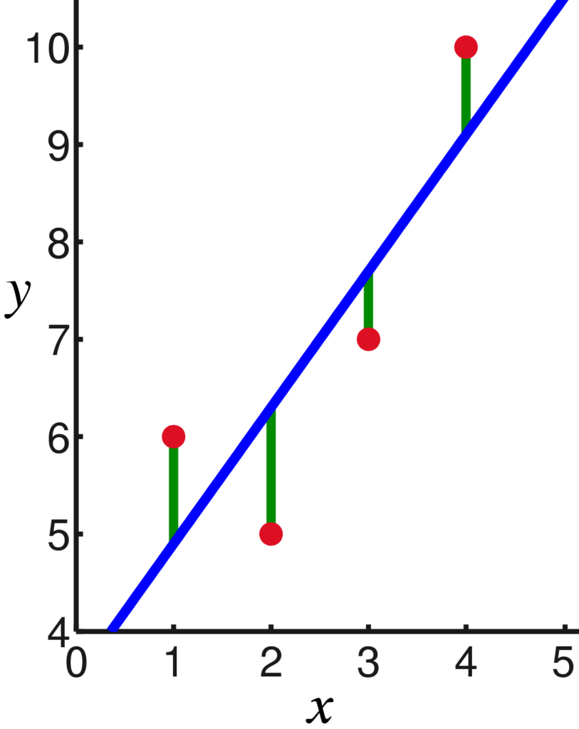
More specifically it minimizes the sum of the squares of the differences, meaning it penalizes bigger differences by more. The smaller the differences, the better the model fits the data. The resulting model can be expressed by a simple formula, especially in the case of a simple linear regression, in which there is a single regressor on the right side of the regression equation.
OLS isn’t the only estimator and it isn’t always the best estimator to use, but it’s the most popular and works in many situations so it has become the defacto standard. There are a few assumptions that are required to ensure OLS is the best estimator to use, and much of the work of a statistician or data scientist in using linear regression is in manipulating the data or updating the model to satisfy those conditions.
Assumptions of Linear Regression
Linear regression is a good default algorithm to use, but it isn’t the best in all situations. It makes four important assumptions about the data. If one or more of these assumptions are violated, then the results of our linear regression may be unreliable or even misleading.
1. Linear relationship: There must be a linear relationship between each input variable, x, and the output variable, y.
2. Independence: The errors – the difference between predicted and actual values – must be independent. For example there must be no correlation between the errors on consecutive days in a time series model.
3. Homoscedasticity: The errors have constant variance at every level of x. When this assumption doesn’t hold you tend to see a ‘fanning out’ of errors over time.
4. Normality: The errors of the model are normally distributed. I.e. they follow a ‘bell curve’ distribution when you plot them.
There are many techniques for dealing with violations of these assumptions. For example if one of your x variables doesn’t have a linear relationship with spend, you can transform the data before including it in your model. That’s quite a common technique when dealing with diminishing returns of advertising. The answer might also be to drop some variables, add other variables in or collect more data.
Bayesian Linear Regression
Traditional linear regression is a ‘frequentist’ approach, where the model is a combination of the x values. Another school of thought is Bayesian, where the regression is formulated using probability distributions instead. The value for y is not estimated as a single value, but instead we get the probabilities for its possible values.
The aim of Bayesian Linear Regression is not to find the single “best” value of the model parameters, but rather to determine the most likely range of values for the model parameters. This can offer more flexibility as it allows us to ‘tell’ the model something we know about the likely range of values to factor in, using model priors. For example with Bayesian Marketing Mix Modeling we can dictate that a marketing channel is unlikely to drive negative sales.
Bayesian methods allow for domain expertise and give us an estimate of the uncertainty in our model. If we don’t have a good idea of the effect of a variable it will have a wide ‘plausible’ range. Using monte-carlo simulation we can factor that in when making predictions, and understand the likelihood of potential future outcomes. This may be more complicated to calculate and use than OLS, but the recommendations better match our intuition and how we actually reason in the real world.
Logistic vs Linear Regression
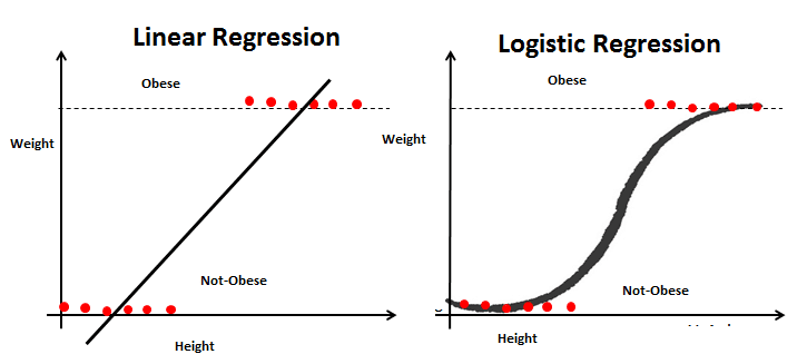
Linear and logistic regression are similar, in that they both use linear equations for predictions. However the functionality is completely different. Linear regression is used for predicting continuous variables, like sales or revenue. Whereas logistic regression is used for classification problems, like predicting whether a user will click on a banner ad, or make a purchase on the website. To do this logistic regression uses the maximum likelihood estimation, rather than ordinary least squares.
Is Linear Regression Machine Learning?
Machine learning (ML) is the study of computer algorithms that can improve automatically through experience and by the use of data, and is considered to fall under the category of Artificial Intelligence. Machine learning is primarily concerned with minimizing the error of a model or making the most accurate predictions possible, which often comes at the expense of explainability.
Linear regression was developed in the field of statistics, but that doesn’t mean it’s not machine learning, as the relatively newer field borrows algorithms and techniques from what came before. Linear regression is considered a supervised machine learning algorithm, because the model learns from the data how best to fit a line between the independent (x) and dependent (y) variables. Unlike many machine learning algorithms, linear regression is quite explainable and easy to use, so it is perceived as a more ‘entry level’ ML technique.
History of Linear Regression
- Legendre publishes the least squares technique in 1805
- Gauss publishes more on the topic in 1809
- Gauss further develops the technique and publishes a version of the Gauss–Markov theorem in 1821
- The term ‘regression’ is coined by Galton in 1885
- Fisher clarifies some of the assumptions needed in 1922
- Economists use electromechanical ‘calculators’ to calculate regressions in the 1950s
Regression methods continue to be an area of active research. In recent decades, new methods have been developed, including Bayesian regression and regression techniques that are robust to different types of data or model assumptions. Most recently regression was involved in developments related to causal inference, which won the Nobel Prize in 2021. We should expect Linear Regression to be with us for a very long time yet.