
One of the core problems to solve when doing marketing mix modeling (MMM) is handling how the results from a previous period ‘carry over’ into the next period. In marketing we know that the full effect of advertising isn’t felt on the same day or week in which the campaign ran. For example a memorable TV campaign might still be driving customers next week, next month, or even next year! Other less emotive and more functional channels like Google Search Ads would perhaps have less of a long-lasting effect.
One way that some modelers approach this problem is to “pre-transform” the input data in order to apply an “adstock” effect to account for this lagged effect of advertising. Modeling this “lagged effect” correctly is critical to the modeling process. Unfortunately, it is quite easy to use these techniques incorrectly, and for the analyst not to realize (let alone the wider business!).
Adstock Definition
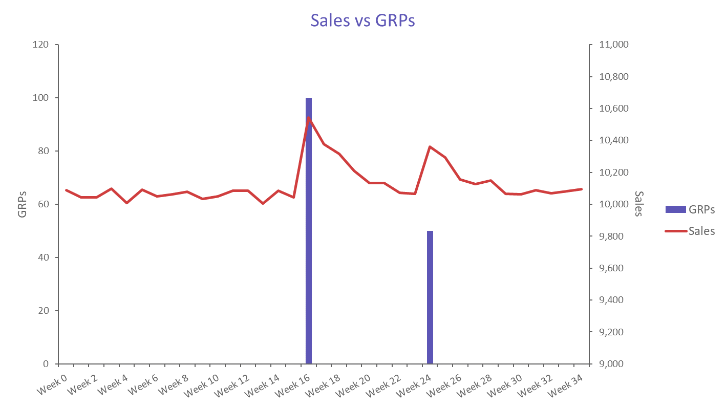
Adstock (sometimes referred to as “carryover” or “decay”) is a concept first outlined by Simon Broadbent in 1979. It refers to the persistence of an advertising effect beyond the period in which the message was delivered. Usually this can be seen in a sales chart as a tailing off of the incremental sales following the period of advertising. The below chart shows GRPs (a TV-campaign specific metric) plotted against sales. Note how each spike in TV ad spend seems to cause a period of elevated sales for some weeks after.
There are a range of underlying phenomena which cause the adstock effect:
- Ad Memorability: The memorability of an advert is an important one – the more emotional the advert, and more engaging the format (i.e. video vs simple text), the greater the likelihood of someone recalling it later.
- Purchase Cycle: Part of the adstock effect may also be to do with the purchase cycle of a product or service – if you see an advert for something that you only buy monthly, it could be a few weeks before you act upon it.
- Channel Mechanism: Alternatively there is the channel mechanism itself – direct mail campaigns take a few days to be delivered and opened.
- Repeat Purchases: There will also be repeat purchases – a new customer for a brand might continue to buy for several weeks, months or years, sales which could theoretically still be attributed to that advertising.
There are other mechanisms, such as word of mouth, social media effects, etc., but the basic idea remains. There will also be factors which effectively reduce the adstock – competitor advertising or promotions, or a poor product experience.
Transformations are often required due to the structure of the model – a simple linear regression model does not allow for anything other than summing together weighted variables. These effects combine and interact so to model the exact effect would be extremely complicated. However, we can make a good approximation quite simply, which can do a surprisingly good job of making aggregate predictions.
Adstock Formula
In traditional MMM, adstock is usually represented by a percentage from 0% to around 95% which denoted how large the second week sales are relative to the first week sales. Note that a 100% adstock would imply that the effect persists indefinitely which is unfeasible. For an example of calculating adstocks, if the advertising results in 1000 additional sales in the first week, 600 in the second week, 360 in the third week, and so on, then the adstock rate would be 60% because each week has 60% of the sales of the previous week. In time-series form, this transformation looks similar to as depicted in the following chart.

Usually “adstock” and “carryover” are synonymous but it is worth noting that some analysts define decay as the complement of adstock/carryover, i.e., decay = 1-carryover. This means that a “70% carryover” may be equivalent to a “30% decay”. This can cause some confusion because the amount of decay is often the amount that is lost between successive weeks rather than the amount that persists. So in our previous example, it would be a decay of 40% because 40% is lost from week to week.
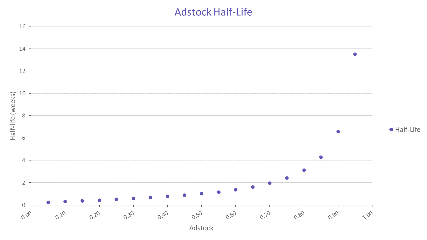
Adstocks can also be described in terms of their “half-life”, the length of time it takes for the incremental sales to decay to just half of what they were in the first week. If an adstock is 50%, then its half-life is 1 week. As adstock gets higher, the half-life gets higher too, but much faster than you might expect. A 70% adstock has a half-life of two weeks, while a 90% adstock has a half-life of almost seven weeks.
If you are the client and you’re not sure about the definition in use then ask the analyst to clarify. If you are the analyst, then be clear what definition you are using, and make sure that everyone in your team is using the same definition.
Adstocks by Market
For any given category, brand or market segment, or type of media used, all the above causes will be present to different degrees. For example, in the car market purchase cycles are quite long and short-term repeat purchases (within weeks or months of the advertising) are very rare.
For fast food, some people will be very frequent purchasers while others won’t. Some categories have a greater proportion of “switchers” which means a brand might get a large short-term impact but one that doesn’t last very long as the people who were your new customers have been attracted by another brand’s advertising and switched to them.
The more brand loyalists that there are in a category (e.g., cars) or the more loyal a brand’s consumers are (e.g., Apple), the smaller the short-term impact of advertising is likely to be (because there are fewer switchers).
Adstocks by Channel
Critically, it should be observed that the media itself does not itself “have” adstock. Adstock arises as a complex interaction between advertising, the audience and the consumers. Some studies compare adstocks of different media types across categories. This can sometimes be misleading as the category itself has an impact upon the adstock, however we do find that certain channels tend to have longer lasting effects than others.

Newspapers could be expected to have a shorter adstock than magazines because a newspaper is disposed of at the end of the day whereas a magazine might hang around in a house for weeks, months or even years!
Because of this variation, it is too simplistic to say that a higher adstock is always better than a lower one. The most important measurement is the total number of sales that result from the advertising, not the period over which these sales were gained.
In most analyses, there will be considerably more “adstocked spend” in the series than there was actual spend. This is because analysts will tend to sum up all the adstocked weeks together with the original media, so there is a cumulative effect of sustained investment. Also, the results from the model will pertain to “adstocked spend” not actual spend, which must be remembered for any subsequent analysis – for example you have to work backwards to get your true cost per purchase or return on ad spend, which is explained in the next section.
When modelling multiple media types across the same period (as is often the case with integrated campaigns), some analysts may decide to just fit the model for TV and then decide that the other media types don’t go into the model. This is an impulse that should be discouraged. It is important to test variables in combination with different adstocks. Large adstocks on TV can exacerbate this problem as media with a more constant presence – magazines, outdoor – can “disappear” under the long tail from TV.
Calculating Adstocks
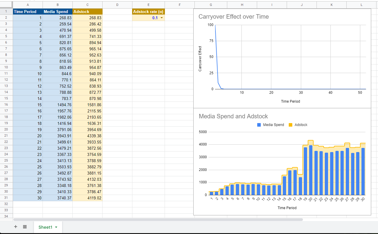
If you’re not interested in math, feel free to skip this section. We also have an Adstock Google Sheet Template that shows how to calculate Adstocks, which you might find more intuitive.
The following are some of the most common methods of calculating adstocks. The approach laid out in this article is not reflective of how Recast approaches it. The actual model specification can be found in the technical model specification.
Still, it’s valuable to see how others solve for this:
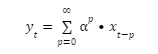
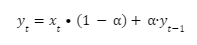
The most common model, as described above, can be formalized as a geometric series, with α as the adstock rate:
Which can be also be represented as
Infinite series are somewhat cumbersome, however, and so with a bit of algebraic manipulation, we can derive the following form:
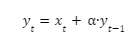
You will, of course, have to set an initial condition at your first data point of simply y0=x0 (or if you have an estimate of a pre-existing adstock level, you can add that in as well, but this is quite rare).
As it turns out, the total number of adstocked GRPs that will be created in the series is readily calculable as well.
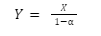
Where Y is the number of adstocked GRPs and X is the number of raw GRPs.
Therefore, as an option, the series can be normalized:
This can be quite useful in calculating, for example, the total number of items sold per million impressions, or equivalent, without worrying about the impact of the adstock. However, this may not be appropriate for all pieces of analysis. In particular, diminishing returns should be applied prior to this step (which will be covered in the subsequent post on that topic).
If you want to calculate the half-life that a particular adstock results in, you can use the formula:

As can be seen in the following chart, the half life increases rapidly with higher adstocks – this is why adstocks greater than 0.9 are quite rare in models.
So how do we arrive at 0.9? How do we know that it’s not 0.2, or 0.5? This process is called hyperparameter optimization, and it’s not an easy subject to broach. In short, traditional MMM vendors will do this part manually, selecting different levels and seeing how that changes the model. If changing from 0.5 to 0.6 hurts model accuracy, or makes some of the other model coefficients implausible or insignificant, perhaps 0.5 is the right level.
This is a multi-objective optimization problem with no easy solution, because each parameter you change affects every other parameter in the model. More sophisticated modeling techniques utilize evolutionary algorithms (like Robyn’s Nevergrad) or Bayesian Markov Chains (like Recast’s solution) to do this work automatically, building 10s of thousands of potential models while evaluating the best tradeoffs.
Unfortunately, the process of hand-selecting these adstock parameters can be error-prone or, even worse, can allow for the person doing the selecting to “shape” the results of the model to what they want to see. There have been stories of modelers who choose a set of adstock parameters not because it gives the best model, but because that model made TV spend look the most effective.
Other Adstock Transformations
Although this model of adstock is by far the most common in practice, it is not the most sophisticated, and isn’t always suitable for all types of media for all categories.
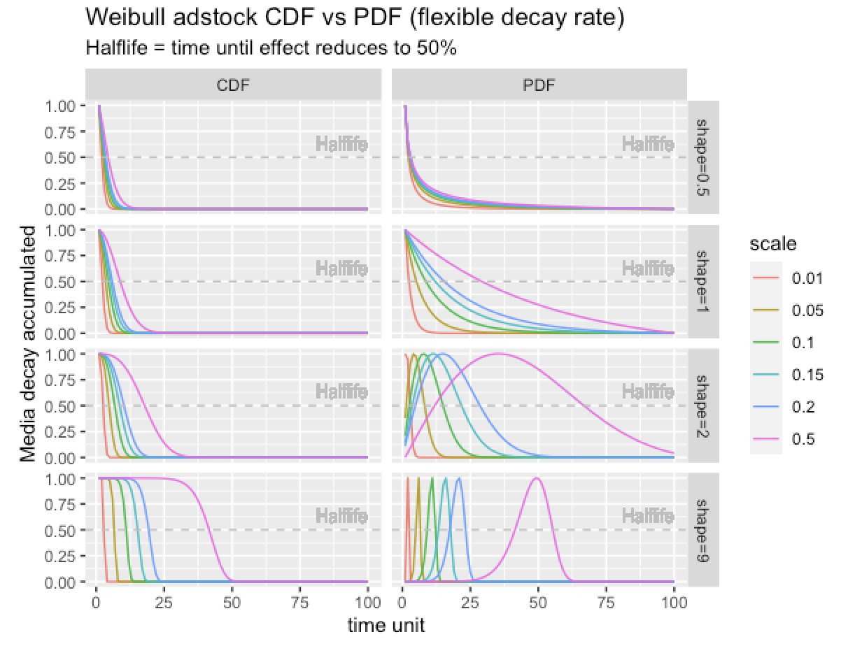
Other libraries like Meta’s Robyn use a Weibull distribution, and at Recast the team uses a negative-binomial distribution to model this effect. This is a more flexible approach that allows for more parameters, including the shape of the curve and scale. Some Weibull Adstock approaches and other distributions also allow for an initial lag to be incorporated.
One practical hand-crafted example was a model that I built of TV licence renewals in the UK. At the time, the primary means of reminding people to renew was direct mail (DM) – the BBC (the British National TV Licensor) would typically send out up to six reminder letters. The response to these letters, in terms of the recipient renewing, did not follow a simple decay pattern. Most people would receive the letter and then act on it sometime in the next month, often peaking at around three weeks after the DM drop date. By means of DM tracking, the BBC were able to provide the exact response rates for each of the six reminders. A simple adstock would be of no use, but a Weibull-distributed response applied to the DM produced much more accurate results.
Magazines might also benefit from a more sophisticated model, as they will be purchased across the circulation period rather than having a single “drop date”. A monthly magazine might not hit peak circulation until week two or three and, even then, it might remain in a household for some weeks or months thereafter. Outdoor can work as an immediate reminder but the effects tend not to persist much past the date that it is visible. When modelling TV, on the other hand, a simple decay usually suffices – It is often easy to pick out because of the large number of people who have been exposed.
To apply a transformation of this type requires the use of a mathematical operation called convolution, together with some sort of research or theoretical justification for the transformation to be applied. This is beyond the scope of the current article, but I may return to it in a future post.
By using transformations appropriately, you can extend the usefulness of the model specification to encompass problems which would otherwise require a different technique to be used.
More sophisticated types of model, e.g., Agent-Based Models, might allow for data in its raw form to be entered directly, depending on how it has been specified. They will often use transformed data, though, if it allows simplification and greater efficiency in the calculations.
Conclusion
Hopefully, this post has given you a much greater insight into the use of the adstock transformation in Marketing Mix Modelling. Using it correctly is an essential part of producing reliable models that properly represent the real-world impact of advertising. Using the wrong adstock assumptions can lead to inaccurate or implausible results, meaning that you’ll make incorrect decisions about where to allocate your marketing budget.
To correctly specify any transformation we need to ask three questions:
- What does the raw data represent?
- For inclusion in the model, what would the variable ideally represent?
- Is there a way in which the raw data can be transformed into a satisfactory representation of the ideal variable?
Only in rare cases can a variable be simply transformed into the ideal variable. More often we need to recognize that we are making a compromise. It is easy to pretend that no compromise is required (e.g., by changing the real question to a slightly different question) but this is a mistake. It is better to have a full understanding of where the shortcomings are in the model to protect against interpreting it wrongly.