One commonly asked question from clients just getting started with Marketing Mix Modeling (MMM), is how much data they need to build a model. It’s a particularly important question in B2B, where there isn’t always the volume that large scale consumer brands enjoy. In theory there’s no ‘right’ answer to this question, because like most questions in statistics, the answer is ‘it depends’. That’s not a particularly helpful response to a busy executive trying to understand if MMM is a viable marketing attribution method for their brand.
So here’s a short answer first, and a longer, more-theoretical answer later.
Short answer: At Recast, we keep it straightforward:
Recast just needs to ingest a simple table: one row for each day, one column per marketing channel, diligently tracking daily spend.
Recast ingests this table plus the outcome variable the business cares about (total revenue, total revenue from new customers, etc.).
Every marketing channel, whether it’s Google Shopping, radio, or TV, requires precise tracking to optimize spend effectively. So it’s very important that you begin keeping a history of all your marketing data, especially for channels like affiliate or podcasting that lack in-platform tracking.
Now, the backstory and what we’ve seen other MMMs need:
Note that this isn’t necessarily how Recast approaches assessing data requirements for marketing mix modeling. The actual model specification can be found in the technical model specification.
When we’re building a model, we’re doing our best to estimate how the real world works. Crucially, we don’t actually know the truth about how our marketing is performing. If we did, we wouldn’t need to build a model in the first place! We have statistical tests and accuracy metrics to guide us, but it’s perfectly possible for a model to be statistically valid, impressively accurate, and still be completely wrong! If Turkeys could do statistics, they’d be very confident in predicting their own odds of survival – and they’d be right – all the way up until Thanksgiving! If you don’t have a good model of the real-world process that is generating the data you observe, you risk being catastrophically wrong.
How do we determine how much data a model needs to be correct, when we don’t know what the correct answer actually is? In situations like this, researchers turn to an elegant approach called “Parameter recovery”. In real world datasets we don’t know the true performance of marketing. If we generate the data ourselves however, we know what parameters we used when simulating marketing performance. If we test different modeling approaches with these simulated datasets, we can see if the models ‘recover’ the parameters, and that tells us something about their correctness. For example if I generate data dictating that Facebook ads have a $4 Return on Investment (ROI), I can simply check how close the model got to $4 ROI to check its accuracy.Building 24 marketing mix models
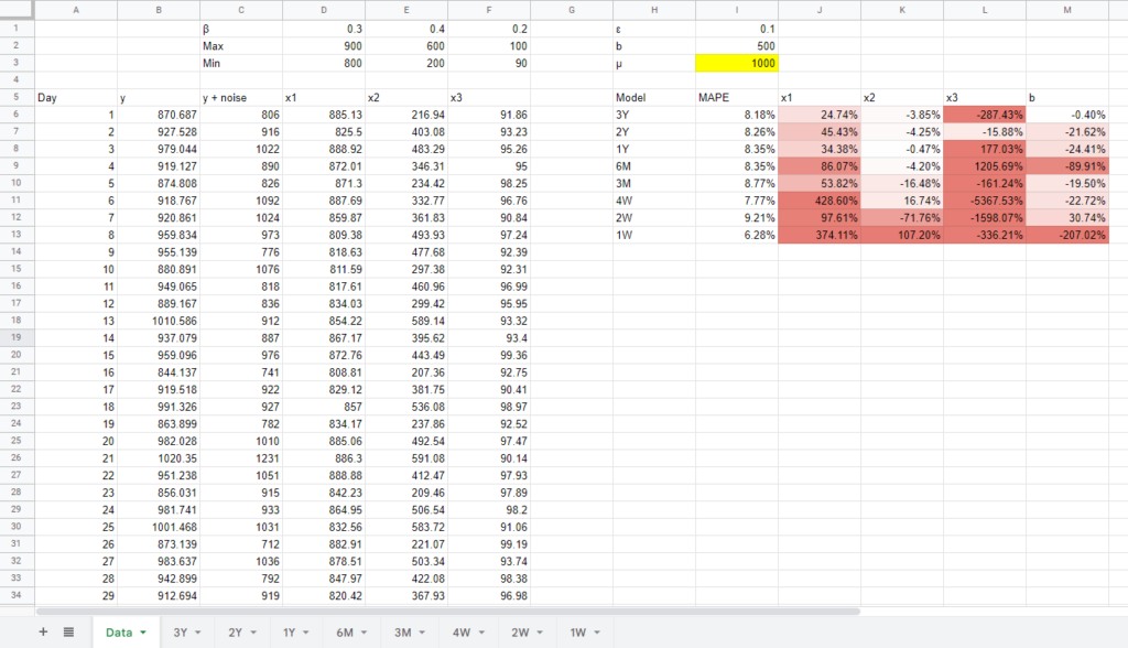
In the context of our question “how much data do we need to build a marketing mix model?”, we can use parameter recovery to simulate what happens to the model when we supply it with more or less data, and see at what level it fails. So that’s exactly what we did: we simulated datasets for 24 different models so we can see how they performed. For each model the underlying performance of 3 marketing channels was the same, the only difference was the amount of data (from 1 week up to 3 years) and the scale (from $100s spent per day to $10,000s). The results of these simulations show that a lot of the normal concerns around data volume are largely unfounded.
The generally accepted way for scientists to determine the effectiveness of a marketing mix modeling technique is to simulate data and then see if we can recover the parameters. This is necessary because with real-life data we don’t actually know the ground truth – what the true underlying performance of marketing is – as all marketing attribution techniques are just different ways of estimating it, with their own strengths and weaknesses. We’ve taken that approach here, by generating data for three marketing channels (X1, X2, X3) and sales (y). You can download the data here:
We used a typical marketing mix based on our experience, which is 3 media channels, with one relatively dominant and stable channel, one higher performing channel that is scaling spend up and down more, and a third with a relatively low effect and small budget. You can think of the first channel as either Facebook or Google ads, the second as a new channel you’re testing like TikTok or Amazon ads, and the third as a channel that does ok but not great, so you just leave it running like Bing or Pinterest.
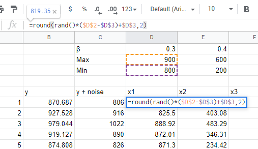
In each case we generated the data using a simple `RAND()` function in gsheets, which gives a number between 0 and 1, and then scaled it based on a min and max we set above. For example, in the model where we’re spending 1,000s per day (represented by the `µ` parameter), we take the random number generated for channel x1, then scale it up so it’s between 800 and 900. We do it in this way so that we can see how the same underlying relationship shows up in the model when we’re spending 10s or 100s per day, or if accuracy improves when we spend $10,000s or $100,000s per day by changing `µ`.
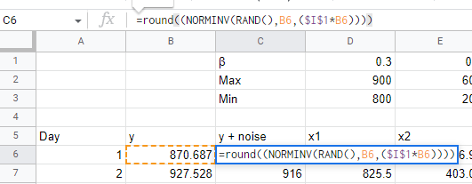
To generate our y variable, which in a real model might be sales, new users, or leads, we calculate it using the `β` values that we decided above, plus an intercept value `b` that represents the number of sales you’d get with no marketing spend. In this scenario we decided that channel x1 should get 0.3 sales / users / leads per dollar spent (1/0.3 = $3.33 CPA), with channel x2 performing better (1/0.4 = $2.50 CPA) and channel x3 performing worse (2/0.2 = $5 CPA). We also added some random noise with a 10% deviation of the mean. We do this with the `NORMINV` function in GSheets, which gives us normally distributed random noise around the sum of the channel contributions.
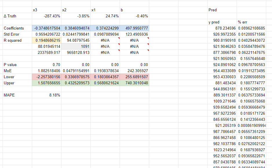
We generate 3 years worth of data (1,095 days) but each model looks at a different subset of the overall data to see how well they perform. Each tab is a new model using the `LINEST` function to do a simple linear regression. We show the MAPE – a measure of error (lower is better) – and a `Δ Truth` row which is the difference between what we know the true coefficient is for a channel, and what the model found. Usually you’d want to use ‘out of sample’ MAPE, meaning data the model hasn’t seen before, but we just used in sample accuracy for expediency.
No simulation is a perfect representation of reality, but this should be good enough for our purposes. In particular, we’re making a number of simplifying assumptions in this model:
- There’s no seasonality
- Channel performance doesn’t change over time
- There’s not declining marginal efficiency of spend (saturation)
- There’s not time-shift (“adstocking”)
- There’s no correlation in our marketing spend
- + more!
You could make a copy of this spreadsheet and change these around to reflect your own assumptions, but you should still get relatively similar results. Note that because we use the random function, it’s recalculated every time you change something in the sheet, so it won’t line up exactly to the screenshots we’ve included here, but should be similar in principle when you try out new numbers.
This is a simplification of reality, and we’d get different results if we use a more complex data generation procedure. As mentioned, we haven’t included seasonality here, which would make having multiple years of data much more beneficial, to tease out that seasonal trend. We haven’t looked at the possibility that marketing performance improves over time, which could be an important factor for models using time-varying coefficients like Uber’s Orbit model (and Recast!). We also assume marketing channels aren’t correlated with each other, don’t get saturated at higher spend levels, and don’t have a lagged effect on performance, which are all typically important for MMM and would add a lot of noise to the analysis.
How many days worth of data do you need for MMM?
We’ll start our exploration based on a brand spending $1,000s of dollars a day, or about $30k a month, $340k a year. This is usually in our experience when brands start getting more serious about marketing attribution, migrating away from last click performance as measured by the platform via tracking pixels or in their analytics with URL parameters.
There are two ways an MMM could be ‘wrong’. You could have a high MAPE, which is the percentage wrong the model was on any given day. You could also have implausible coefficients, meaning the model got a channel’s contribution wrong, which would cause you to allocate too much (or not enough) budget to that channel. We’ve reported on both for the purposes of this analysis.
The main interesting takeaway from this data is that the MAPE is relatively unchanged. We know we added 10% noise to the data (plus some noise from rounding), and our MAPE hovered around 8% for all models. Even when we got down to less than 4 weeks worth of data the error wasn’t significantly higher and depending on the luck of the random function, we often get lower error for smaller date ranges! Note that it’s possible for a model to be broadly predictive in terms of accuracy, whilst still being implausible (getting the coefficients wrong), which is one of the things that makes MMM so hard.
This would be different if we had included seasonality in the data, because models that had a few years to tease out the seasonal trend would perform far better. However, shorter models would have performed better if we had baked in a significant change to our marketing performance in the past few months, because past data would be less reliable. The takeaway is that if seasonality isn’t a big factor for you, or if your past data isn’t really relevant for some reason, you shouldn’t feel too uncomfortable using a smaller dataset, like the 3 to 9 months recommended by Meta.
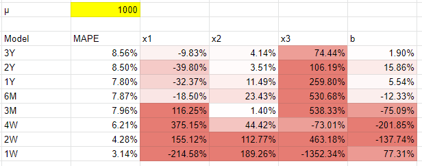
The real problem with small datasets wasn’t overall accuracy, but parameter recovery. You can see with less than 3 months data the x1 estimates got really far off. With the x2 channel we saw far better estimates, because that channel had a lot more variance: spend was as low as $200 and as high as $600. We could correctly estimate the performance of this channel within a few percentage points of error with at least 6 months of data. So it’s the variance in a channel that matters, not just the number of observations.
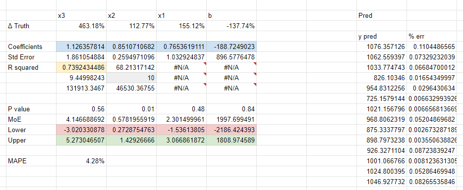
The x3 channel had similar variance to x2 but suffered from small effect size: with less than $100 spent per day it didn’t show up as significant in the model. Depending on the numbers you get from the random functions, it either gets gobbled up by the other channels, or the intercept. The rule of thumb is to have at least 10 observations per variable (including the intercept), so with our simple model we could get away with 10 x 4 = 40 observations, or just over a month’s worth of data. In practice we would say using 3 to 6 months data for most small advertisers spending just over a thousand dollars a day with a simple marketing mix would be a safe bet.
Do you need to be a big advertiser to do an MMM?
Another common misconception we hear a lot is that you need to be a Fortune 500 advertiser to build a marketing mix model. Actually the eagerness of public companies to adopt MMM comes from the cost of building a model, and the introduction of the Sarbannes-Oxley Act in light of the Enron scandal, which dictated more justification for large expenses. Now with iOS14 breaking digital tracking and changing the attribution landscape, as well as the introduction of open source libraries, and software as a service tools like Recast, the cost is coming down and MMM is being democratized.
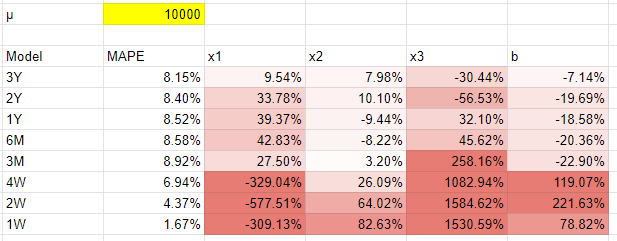
We made a copy of our existing template and changed the `µ` variable to 10000, i.e. $10,000 dollars a day, but we left all the underlying marketing performance the same (here’s our data, if you do the same you’ll get different numbers due to the random functions). In doing this we found there was no real impact on accuracy! MAPE was consistent across all models. We tried this multiple times with new generated random numbers and there was no real difference. Higher marketing budgets, all things being equal, didn’t change the accuracy of the model.
However the big takeaway and clear trend was that with more data you get better parameter recovery, with better results for x1 and x3 channels at this higher spend level. However larger businesses have more complex marketing mixes, and need to include more variables in their models, so risk falling foul of the 10 to 1 observations to variables rule of thumb. They also tend to have in our experience more fixed budgets, planned quarters or years in advance, so are prone to less variance in their spend, another issue counteracting this boost in parameter recovery. So what about going the other way? Can smaller businesses spending $100 a day (µ = 100) get value out of MMM?
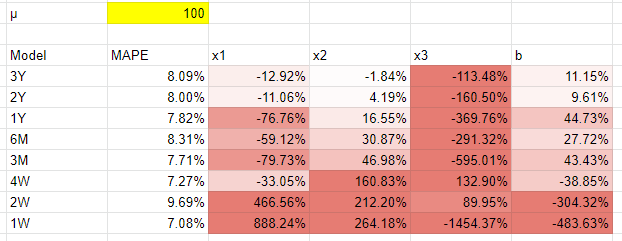
Our simulation says that they still can (link to data here, or make a copy of the template and change the µ variable to be 100). The random number generator really varies the result, but we ran this multiple times and quite often the coefficients for at least the x2, x1, and intercept variables were within reasonable margins of error with more than a year’s worth of data. The real loser in this scenario was channel x3, which was spending less than $10 a day at this level. We would say that is pretty much the theoretical limit below which marketing mix modeling just can’t work well. Though the practical limit would be far higher given the time and money it can cost to build an MMM, versus the relative benefit of allocating your marketing budget 10-50% better via the model.
One thing that stands out is that the accuracy was still pretty good: no real difference to the higher spending brand’s models. Small businesses can far easier vary their marketing spend by day – often it’s the founder themselves making changes – so they can easily make each channel look like x2 by increasing or decreasing the budget over time to give the model more to work with. That means that a small business can theoretically have the same or better predictive power as a fortune 500 company, so long as they have access to the time / money / technical expertise to build a model.