Is there a good way to do a test of statistical significance for ROAS?

Someone posed the following query in a marketing measurement slack I’m in:

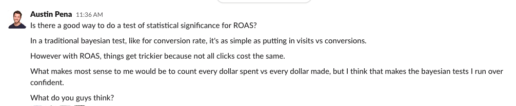
At first, this question seemed really easy. Hubristically, I replied “just use a t-test for difference in means.” However, it turns out that the analysis isn’t quite so straightforward (which I realized after a few minutes of thought and some sharp questions from the original question-asker).

The reason why it’s not straightforward is because:

• We’re asking a question about the relationship between two variables (spend and revenue) which is different than a traditional t-test where you’re looking at the difference in one variable (e.g., revenue) between two groups.
• It’s not obvious what the right unit-of-analysis is. What’s an “observation” in this analysis?
• There’s no natural standard-deviation reported by google analytics (or whatever) so it’s not clear how to calculate the t-statistic.

So to solve this problem, I did what I normally do: I turned to google sheets to generate some fake data. You can see how I generated the data at this link (and make a copy to play with this yourself)

Here’s the data I generated:

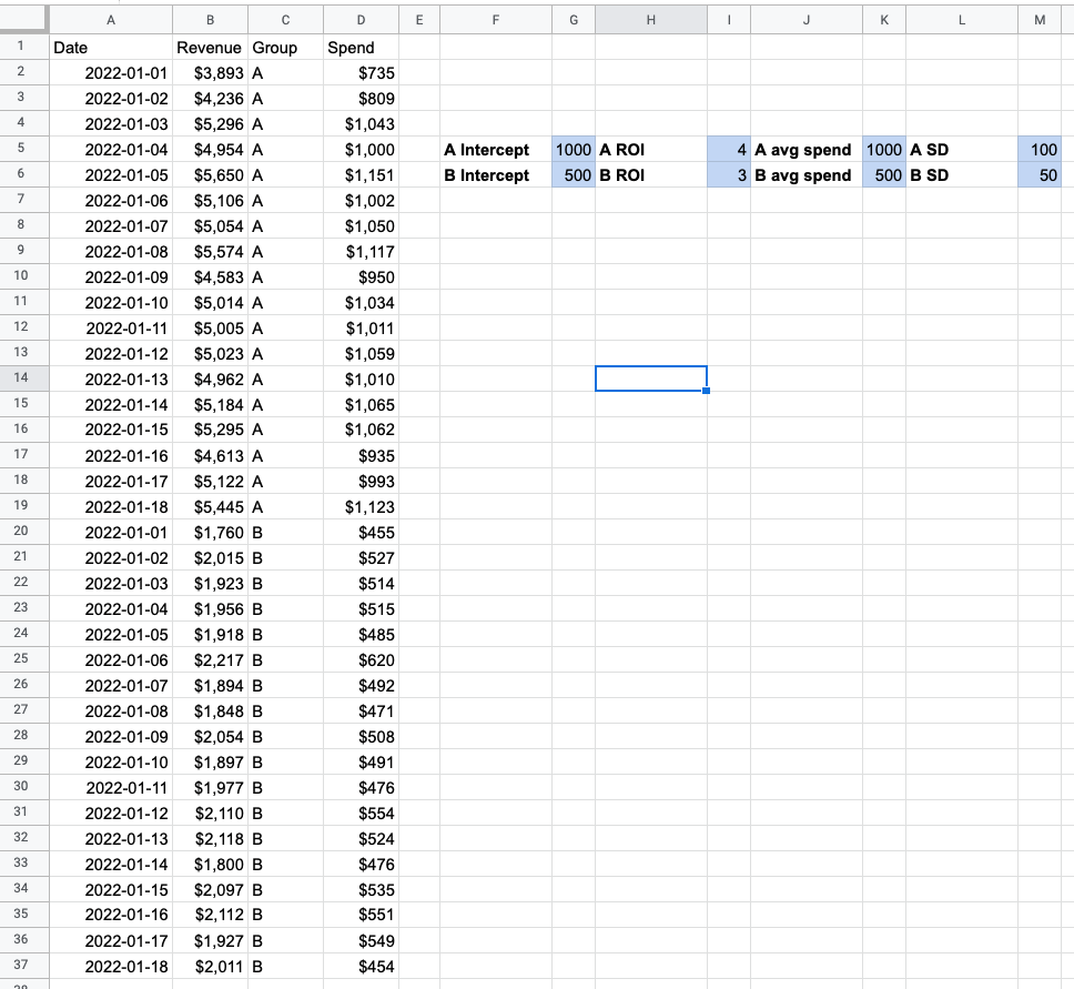
The fields highlighted in blue are the “inputs” that I used to generate the data. The true ROI for group A is 4x and the true ROI for group B is 3x. The other parameters mostly have to do with the other random or fixed parts of the system.

I downloaded these data as a csv, loaded them into R, and then ran the following code:

m <- lm(Revenue ~ Group*Spend, data=df)
summary(m)

This is a linear regression where I’m controlling for date (since there are two observations per date, one for each group), the group effect, the spend, and the interaction between the group and the marketing spend.

Here’s what the output looks like:

Call:
lm(formula = Revenue ~ Group * Spend, data = df)

Residuals:
    Min      1Q  Median      3Q     Max
-184.33  -60.86    8.12   57.70  165.01

Coefficients:
             Estimate Std. Error t value Pr(>|t|)
(Intercept)  1111.173    131.244    8.47  1.1e-09
GroupB       -267.911    237.432   -1.13  0.26755
Spend           3.893      0.128   30.35  < 2e-16
GroupB:Spend   -1.565      0.414   -3.78  0.00065

Residual standard error: 83.6 on 32 degrees of freedom
Multiple R-squared:  0.998,     Adjusted R-squared:  0.997
F-statistic: 4.29e+03 on 3 and 32 DF,  p-value: <2e-16

Unfortunately, the output here is quite noisy but we care about exactly one line of output here:

GroupB:Spend   -1.565      0.414   -3.78  0.00065

This is telling us the estimated coefficient, standard error, t value, and p-value for the GroupB*Spend interaction term. The p-value from this term is the p-value for the difference in ROAs between our two groups!

In this case, since we’re:

• Looking at group B and
• The coefficient is negative and
• The p-value is <0.05

We can say that group B has a statistically significantly lower ROAS than group A.

However, there are a few implicit assumptions we’re making with this analysis that I want to highlight here since they might not apply well to your business:

• Group A and Group B are totally independent (i.e., there’s no impact of marketing to group A that’s impacting group B)
• There’s no over-time effects (i.e., there’s no “adstocking” effects)
• The correct unit of observation here is a day’s worth of marketing performance (and all days are basically the same)

And that’s it! We’ve seen that we can use a linear regression with an interaction term to estimate the difference in ROAS between two different ad campaigns.

Of course, if you want to build a more sophisticated model (to control for holidays, day-of-week effects, etc) you definitely can, but this simple analysis is most closely mimicking the assumptions of the t-test. It turns out that in fact many statistical tests can actually be generalized to a linear-model framework, which you can read more about here.