Counterfactuals: A Practitioner’s Guide

In this article:

• What is a counterfactual? – Intuitively understand the concept of counterfactuals
• Counterfactuals in marketing measurement – How this applies to measuring the impact of paid media spend
• Why RCTs are the gold standard – And why they’re nearly impossible to implement in the context of marketing
• Three techniques for building counterfactuals:
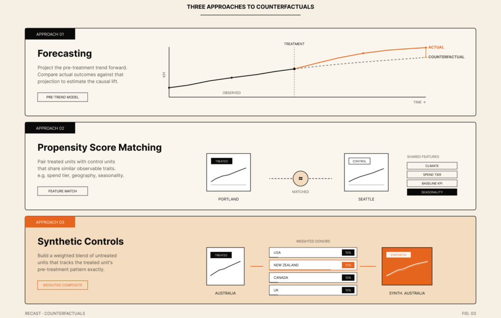
  • Forecasting – Using predicted outcomes as your baseline comparison
  • Propensity Score Matching – Finding statistically similar markets based on shared characteristics
  • Synthetic Controls – Constructing a weighted blend of markets to create a near-perfect comparison
• How to choose your approach – The trade-offs between methods and when to use each

By the end, you’ll have a deep and practical understanding of counterfactuals, including how to build and evaluate them for your own marketing tests.

All the code and sample data behind the forecasting and propensity-score-matching examples in this guide are available on GitHub so you can run the methods yourself.

What is a counterfactual?

You’re in the market for a new job, find a great opportunity, and submit your application. But you don’t stop there. You also network with the hiring manager on LinkedIn, call in a favor with someone who knows the CEO, and send thank you emails after every interview. A few weeks later, you get the offer!

But after all of this work, you naturally wonder: would I have gotten the offer without all that extra effort?

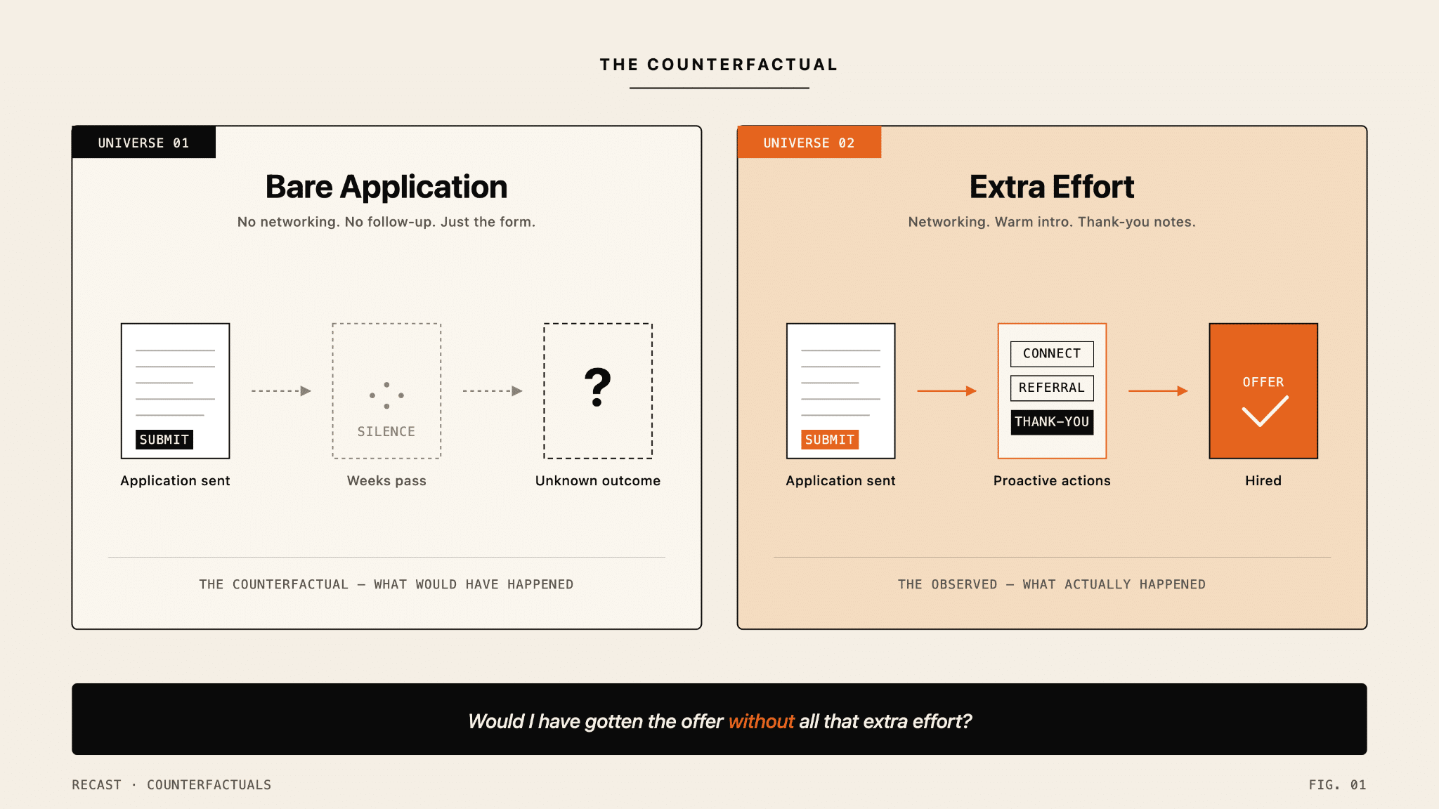
That’s a counterfactual — what would have happened if you hadn’t intervened beyond the application you submitted. You have the observation (got the job) and the intervention (networking, thank yous), but the only way to know if the intervention mattered is to observe what would have happened without it. And in this case, you never can.

Counterfactuals in Marketing Measurement

In the marketing world, we face a similar problem when we make a change to our marketing strategy. If we raise our spend in display channels, for example, we might expect to gain additional revenue. After doing this for 4 weeks, we indeed observe an increase in our revenue. You do a little happy dance and then confidently advocate for an increase in the display budget for the next quarter. But how do we know that the extra spend is the actual reason for the increased revenue and that we wouldn’t have obtained that revenue anyway without the extra spend? 

It’s tempting to accept the increase in revenue at face value and to attribute this to your increased display ad spend. That’s what you expected would happen anyway, right? But what if you’re wrong? What if all that additional revenue would have occurred even if you had held display spend steady? If that’s the case, you just wasted precious marketing dollars. Even worse, you just advocated for a budget increase for this channel. If you’re wrong, you’ll notice when the quarter wraps that the anticipated lift from your additional display channel never materialized and that you’ve wasted piles of cash on an ineffective marketing strategy. 

Avoiding an outcome like this requires a strong counterfactual. We want to know what would have happened if we hadn’t increased the display spend for those 4 weeks. This is often why marketers run A/B tests to evaluate the effectiveness of additional paid media spend. For example, you may choose to run a conversion lift test for Google Display. You separate your test sample into two groups. If one group is getting increased spend in display (your treatment) and the other is not (your control), you can estimate the effect of the additional spend by observing the difference between the high display spend group and our control group (the counterfactual). This looks a little something like this:

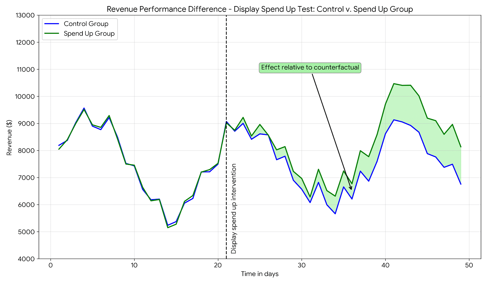
Since the control group (blue) and the spend group (green) were so similar to one another before the intervention, we can be reasonably confident that the difference between them during the intervention period represents the incremental effect on revenue of the additional spend.

RCTs – The Gold Standard?

There’s a broader problem, though. Cleanly matched control groups can be difficult to identify! Your analysis and interpretation of the effect of your spend is only as accurate as the precision of your counterfactual. A poor counterfactual will result in a biased estimate of lift. If your counterfactual is too optimistic (values higher than actual) you may underestimate the effect of your additional spend. If the counterfactual is too pessimistic (values lower than actual) you may overestimate the efficiency of your added spend.

Luckily, there are a number of statistical and methodological tools available to help create reliable counterfactuals even in the absence of an ideal research method. Before we get into that, let’s be clear – the gold standard for a counterfactual is an individual-level randomized controlled trial (RCT) like those used in  efficacy trials for new medical treatments or prescription drugs. In an RCT, the control and treatment groups are selected at random from a broader population, the intervention is provided to the treatment group(s), and then the differences between the control and treatment groups represent the impact of the intervention. Fundamentally, this is still an A/B test, but the randomization process helps drive, in general, more trustworthy and replicable results.

However, individual-level RCTs are nearly impossible to implement in the marketing world. For some digital channels, this may be possible and may even be pretty simple, but for some of your offline channels, you’re out of luck or will need to develop a more nuanced and complex method. Additionally, RCTs may be difficult to implement even for digital channels depending on the level of granularity at which you purchase your media or the specific individual-level tracking policies for your vendors and channels. If you can do an RCT, this will provide you with the most robust learning and the highest probability of identifying causal relationships between your spend intervention and your key performance indicator (KPI). If you don’t have the capacity for RCTs, however, there are other approaches that will work!

Let’s operate under the assumption that you are unable to perform an RCT but that you want to identify the impact of a test that you implement in your display channel. Here are a few ways that you can go about creating your counterfactual if an RCT is unavailable to you:

Let’s do a little deep dive into each before we show you how these work from a statistical standpoint!

Using a forecast as a counterfactual is a relatively straightforward method for comparing your treatment group to your expected outcome. Essentially, you run a forecast on your revenue prior to implementing your spend up or spend down intervention. From there, you compare your actual observations during the intervention period to the forecast’s predictions for that same period in order to calculate incremental lift.

Let’s imagine for a moment that you intend to run a massive company-wide promotion that will impact every market in which you sell your product. Prior to implementing the promotion, you could run a forecast on your expected sales without that promotion. This would look a little something like this:

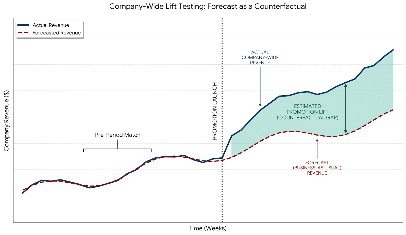
Importantly, you’ll notice that the forecasted revenue was compared to the actual revenue before the promotion launch to ensure a solid and reliable match prior to trusting the forecast as a counterfactual.

This, fundamentally, is one of the biggest weaknesses of this approach. Namely, that it’s dependent on the accuracy of your forecasts. 

If you have a strong, reliable, accurate forecasting engine, using a forecast as a counterfactual is a viable option. 

If, however, your forecasts are weak/unreliable, this method will be very unlikely to give you valid results.

However, this is a good method if 1) you have a strong forecasting engine and 2) the intervention you are implementing is difficult or impossible to control at a more granular level. Running a full company-wide promotion prevents you from selecting control and treatment groups, so a method like forecasting can create a “what do we believe would have happened?” approach to counterfactual generation. Be cautious using this approach and be sure to consider the uncertainty of the forecast in your estimation of the impacts of the intervention you’re measuring. 

Propensity Score Matching

This technique relies on the statistical similarities between your treatment group and your control group. This can happen at the market level or at the user level, but the approach is generally the same: find a match for your treatment group based on important shared behaviors. 

Here’s a practical example – imagine that you are selling fitness equipment and you’re looking to identify the impact of additional B2B sales cold calls that you’re implementing in a handful of cities. Your treatment group has already been selected and, specifically, they are urban cities on the west coast (Portland and San Diego). How would we determine the best counterfactuals? We could use propensity score matching to identify cities that share similar features associated with those target markets:

1. Number of gyms per square mile
2. General weather conditions
3. Baseline sales in the city
4. Number of gym memberships sold per year
5. Geographic region

Something like this would probably result in matched markets that share similar traits to your target markets. It wouldn’t make any sense to pair Portland with Erie, PA. They are vastly different sizes, in totally different geographic regions, and likely have wildly different baseline sales. You would probably end up seeing matches like:

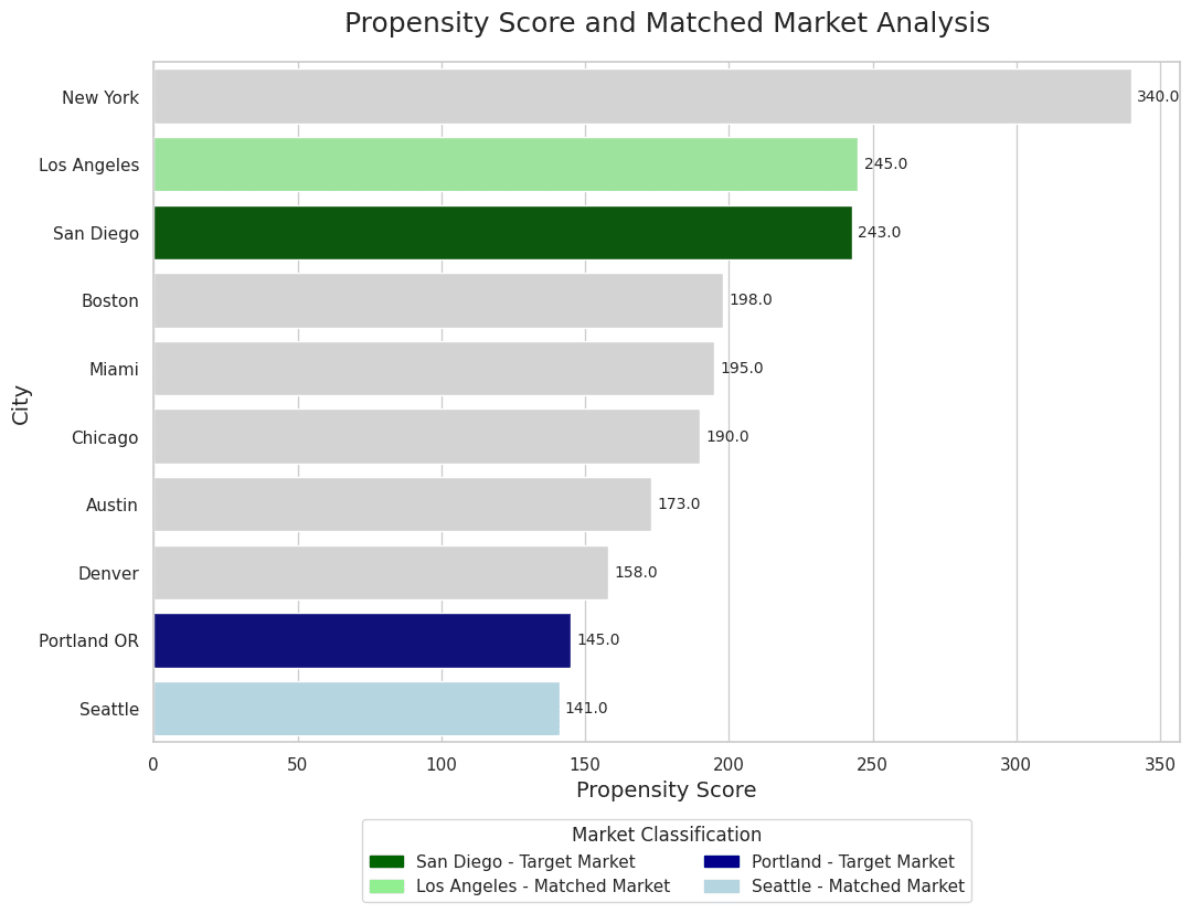
The process for creating a matched market to serve as a counterfactual through propensity score matching can be very simple or very complex. But the overall idea is that the matching doesn’t just happen on pure statistical similarity – it requires measurable similarities related to important factors that drive your business.

This is a relatively intuitive way of choosing a counterfactual. It allows marketing teams to overlay their knowledge about their business and the factors that drive their KPIs with statistically rigorous processes for identifying markets that share high overlap in those factors. The problem is that this doesn’t guarantee a strong statistical match between the control and treatment groups during baseline. Additionally, propensity score matching requires large amounts of data with high fidelity across a diverse set of measurements (imagine how hard it would be to get an accurate measurement of gyms per square mile!). 

Synthetic Controls

While propensity score matching sounds and feels intuitive, it requires a lot of data-intensive thought and testing. Additionally, it doesn’t guarantee a strong match between your control and treatment groups. Enter synthetic controls. This approach takes a different angle to the problem. Rather than attempting to match based on similar factors between markets, synthetic controls focus on creating the most statistically similar control group possible, even if it doesn’t necessarily represent an intuitive match between treatment and control.

Let’s continue with the exercise equipment sales example. If we were to identify the similarities between LA and San Diego using propensity score matching, we might then look at the actual KPI data and see some pretty substantive differences between their performance as markets.

What if, instead of selecting just one market, we selected many markets and weighted their KPI values through simulation exercises to ensure that there was a nearly perfect match between the treatment group and the aggregate KPI in the control group?

Below, you can see an example of what something like this would look like! Let’s say that we’re interested in running a spend up test in New York City. But, New York is a pretty unique place and it might be difficult to find a properly matched market using a technique like propensity score matching. So, instead, we construct a synthetic control by weighting the revenue from multiple other cities such that we’re able to reasonably imitate the revenue in New York City with a high amount of accuracy during a baseline phase. Then, we use the gap between New York and the synthetic control during the spend up phase in NYC to calculate incremental lift:

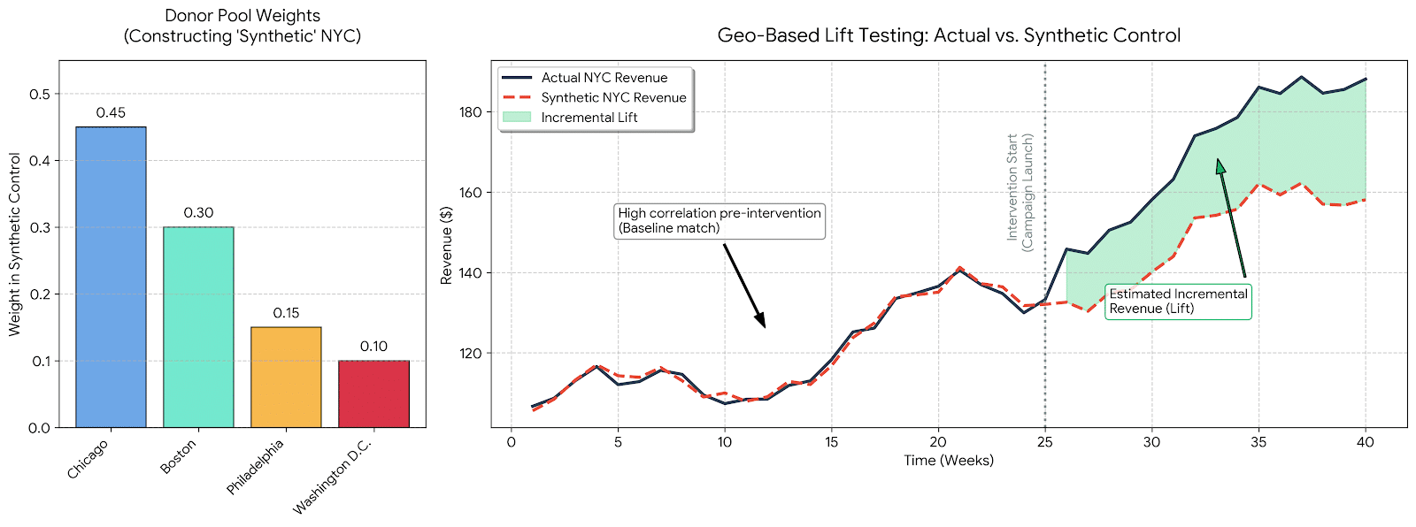
Synthetic control methods are excellent because they are problem-agnostic. In other words, synthetic controls don’t require high fidelity data on exogenous variables like you might need in propensity score matching and they require much less rigorous experimental design and control to be effective. 

The main drawback of synthetic controls is that they don’t hinge on any theoretical relationship between the control and treatment. Rather, they build artificial controls that are statistically as similar as possible without accounting for or even considering other variables that may be similar or different between the treatment and control conditions. This can be difficult to explain to non-technical stakeholders and may engender some skepticism about the propriety of the matches.

Importantly, the three methods shown above are not an exhaustive list, but rather serve as a set of examples for how to think about and implement counterfactual analysis. The goal of counterfactuals, regardless of the method you choose, is to answer the question “what would have happened if I hadn’t changed my marketing spend?” 

Be cautious when selecting your method and, if possible, consider validating your tests using multiple counterfactual approaches to help triangulate your results. While there’s truly no substitution for a well-designed RCT, counterfactual approaches like those detailed above can help you derive meaningful insights from your marketing tests and improve your ability to make strong decisions on your marketing spend.