Many people’s instincts when building a marketing mix model is to include as many control variables as possible. This often seems intuitively correct since many people are taught that “more controls is better” when they learn about regression analysis, but unfortunately the approach is often wrong, and in this article we’ll explore why – including with some code examples you can find here.
Every analyst learns about omitted variable bias early on: if you leave an important variable out of your analysis, your estimates will be off. The lesson sticks, but what doesn’t get talked about enough is the problem of included variable bias.
But including the wrong variable(s) in a model can bias your estimates just as badly as leaving out the right one. Unfortunately, included variable bias can be a huge problem and gets almost no airtime compared to its more famous statistical counterpart.
The core issue here is that variable selection is not a statistical question. It’s a causal inference question. The answer depends entirely on what causes what, or in other words, the causal structure of the system you’re studying.
To show the damage a “bad control” can do, we built two simulated datasets – you can find both here. Simulation lets us do something we can never do with real data: set the true causal effect ourselves. We call this known truth the oracle.
Then we fit two models: a correct specification that controls only for confounders, and a version that adds the bad control. Comparing both estimates against the oracle shows where things go wrong.
The Mediator Trap: Paid Social Prospecting, Organic Search, and Sales
Here’s a concrete example: An analytics team at a crypto exchange is building a model to estimate the effect of paid social prospecting spend on sales (their KPI). They have daily data on their paid social spend, organic search volume, sales, and the price of BTC. Their instinct says “let’s include everything in the model!”
Here’s the causal structure. The arrows show the direction of causation — if A → B, then A causes B. Reading these diagrams is all you need to figure out which variables belong in your model and which don’t.

The variables in this scenario:
- Paid Social Prospecting Spend — daily dollars spent on paid social ads targeted at people who don’t yet have an account (the treatment they want to measure the effect of)
- Organic search — volume of Google searches for the brand name (a mid-funnel metric driven largely by prospecting exposure)
- Sales — daily revenue (our outcome)
- BTC Price — the daily average price of Bitcoin, a market signal that drives both the exchange’s ad-spend decisions and consumer demand for crypto
Paid social prospecting affects sales through two paths. There’s a direct effect — someone sees a social media ad and signs up directly. And there’s an indirect effect — someone sees the ad, searches the brand name on Google, clicks an organic link, and then signs up. Organic search sits on that second path. It’s a mediator, because it carries prospecting’s effect to sales.
Why might the team at the crypto exchange want to control for organic search? Say their analyst opens Google Analytics to investigate where last week’s sales came from and finds organic search, a non-paid channel, appears as a top-converting one. On days with heavy paid social spend, organic traffic to the brand also spikes. So, in trying to separate sales attributed to organic search from the incremental sales generated by paid social, the analyst decides to add organic search as another control variable.
But the Google Analytics dashboard does not show the direction of causation. In this case, organic search is not an independent driver of sales, but a downstream consequence of the paid social campaign.
The price of Bitcoin, on the other hand, is a textbook confounder. It drives prospecting spend (the exchange leans into marketing when the crypto market is hot) and sales (more people sign up and trade when Bitcoin is rising). The analytics team at the exchange should control for it.
We simulated data where we set the true incremental ROI of prospecting ads on sales to 1.2x — meaning every additional dollar of prospecting spend generates $1.20 in sales. Then we tested two models to see which one recovers this “known truth” correctly:
- The correct model, which includes “Prospecting” and “BTC Price” as controls, estimates the incremental ROI of prospecting spend on sales at 1.15x — a deviation from the true effect of just -4.4% from the truth. Controlling for the confounder works as expected.
- The correct model above, but also adding “Organic Search” as control variable, estimates an incremental ROI at just 0.35x – returning $0.35 per dollar spent in prospecting ads — a deviation from the true effect of -71.3%. The estimate of incremental performance isn’t wrong in some absolute sense — it’s capturing only the direct effect of prospecting on sales. But if your goal is the total effect – the impact of prospecting on direct sales and its ability to drive increased Organic Search demand – you just lost over 70% of this impact. Worse, a profitable channel for the business now looks like it’s losing money (ROI below 1.0x).

What happened? By controlling for organic search, the model tried to hold that variable constant, effectively asking “what is the effect of prospecting on sales among periods with the same organic search volume?” But organic search volume is part of how prospecting affects sales. Holding it constant blocks the indirect path. The only effect left is the small fraction of prospecting’s influence that reaches sales directly without passing through search.
This is one of the most common variable selection mistakes in marketing mix modeling. Analysts see that organic search, website visits, or add-to-cart rates correlate with both media spend and sales, and include them as controls. But these mid-funnel metrics don’t confound the relationship — they transmit it. So controlling for them doesn’t remove bias, it changes the effect we are measuring (i.e., direct effect only).
The Collider Trap: Ad Spend, Inquiries, and Sales
Here’s a different scenario. Looking at their data, the team at the crypto exchange now notices that customer support inquiry volume correlates with both their paid ad spend and resulting sales. More advertising means more pre-purchase questions, and more sales means more post-purchase support tickets. An analyst looks at this and thinks: “Inquiries capture demand… I should include it as a control!”
But look at the causal structure here:

The variables in this scenario:
- Ad Spend — daily dollars spent on advertising (our treatment)
- Sales — daily revenue (our outcome)
- Customer Inquiries — daily volume of support contacts, including pre-purchase questions driven by ads and post-purchase tickets driven by sales
- BTC Price — the daily average price of Bitcoin, driving both ad-spend decisions and consumer demand
Inquiries don’t cause ad spend or sales. Both cause it. That makes this variable a collider.
Again, we test two models to estimate the impact of paid media on sales, with a known true incremental ROI of 1.50x ($1.5 in sales per dollar of ad spend). Each model uses a different set of control variables:
- The correct model, which includes “Ad Spend” and “BTC Price” as control variables, estimates an incremental ROI of 1.48x — a deviation from the true effect of just -1.2%.
- The correct model above, but also including “Inquiries” as a control variable: estimates an incremental ROI of 0.9x — a deviation from the true effect of -39.8%. The exchange would conclude that ad spend is losing money (ROI below 1.0x) when in reality it returns 50 cents on every dollar.
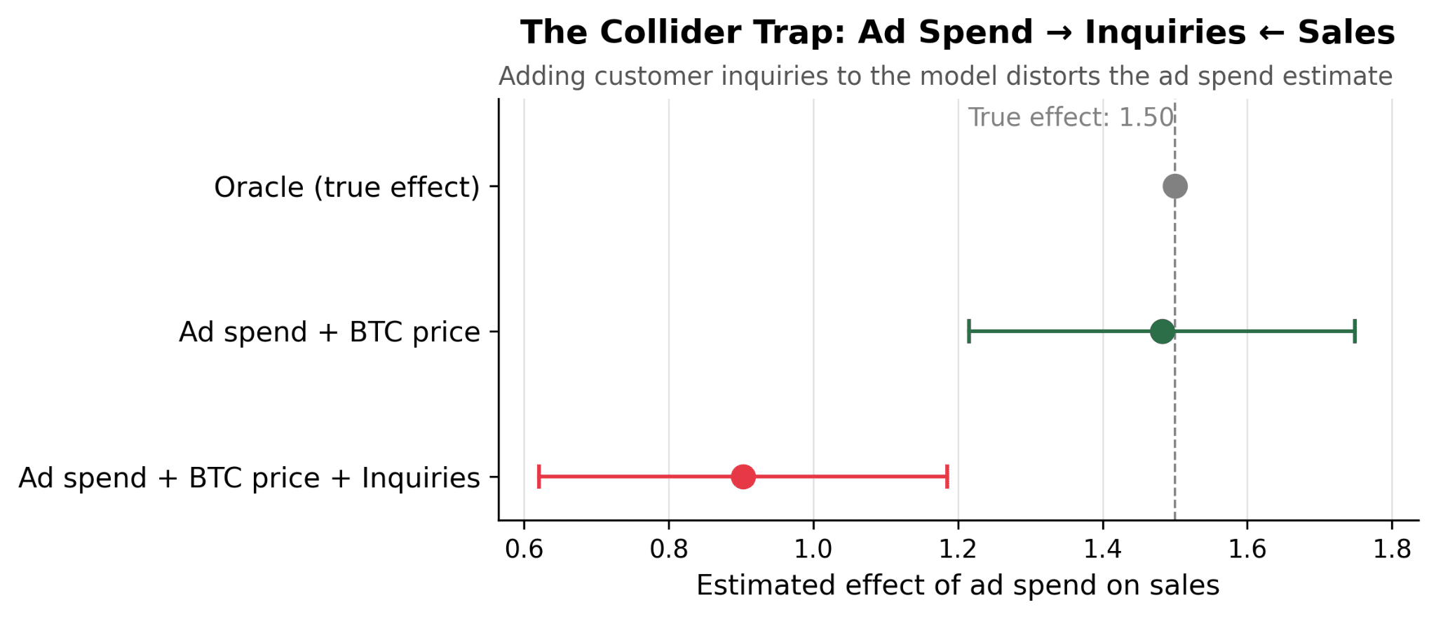
Why does this happen? When you control for a collider, you create a spurious association between the treatment and outcome. Among periods with similar inquiry volume, high ad spend implies lower organic sales (because if inquiries are held constant, one cause being high means the other must be low). That spurious component is entirely artificial — it doesn’t exist in the real data. The model introduced it by conditioning on the wrong variable.
The collider trap is subtler than the mediator trap. Any time you see a variable that is downstream of both your treatment and your outcome — customer satisfaction scores, support tickets, NPS — be suspicious. It probably doesn’t belong in your model.
The bias argument is reason enough to be disciplined about variable selection, but marketing mix models aren’t just used to estimate past effects as above. We also use them to forecast future performance.
At that point, every variable in your model is a variable you need to forecast too, to use as inputs. Economic conditions require a macro projection; organic search requires its own time-series model, etc. So each unnecessary input doesn’t just risk bias, but adds another weak point where the forecast can break, since each forecast carries its own uncertainty.
Same Variable, Different Business
The role a variable plays in a model of marketing performance ultimately depends on the intricacies of that business. The same BTC price time series that confounded the crypto exchange’s marketing model is irrelevant in other contexts.
Picture a regional Heating, Ventilation, and Air Conditioning (HVAC) chain that happens to share the marketing agency with that crypto exchange. That agency tends to move all its clients’ daily budgets in lockstep: when one account ramps up, the others ramp up too. So day after day, HVAC ad spend drifts up and down alongside BTC price.
For this business, the main confounder is actually weather (not crypto, of course). Heatwaves push the chain to spend more on ads and push customers to buy. BTC only touches ad spend, through the shared-agency coincidence, and stops there.
Now suppose the modeler shrugs and tosses BTC into the model anyway because they believe more macro variables won’t hurt and they saw a convincing overlay of sales data with crypto prices. We simulated a year and a half of daily data of this HVAC business with a true incremental ROI of 1x ($1.00 in sales per additional dollar of ad spend), with weather driving both spend and sales, and BTC price moving with spend through the agency channel.
Those are the results of the models:
- Correct model (Ad Spend + Weather): incremental ROI estimate of 1x, with a 95% confidence interval of [0.80, 1.20]
- Correct model + BTC as a contextual variable: incremental ROI estimate of 1x, with 95% CI of [0.75, 1.24]
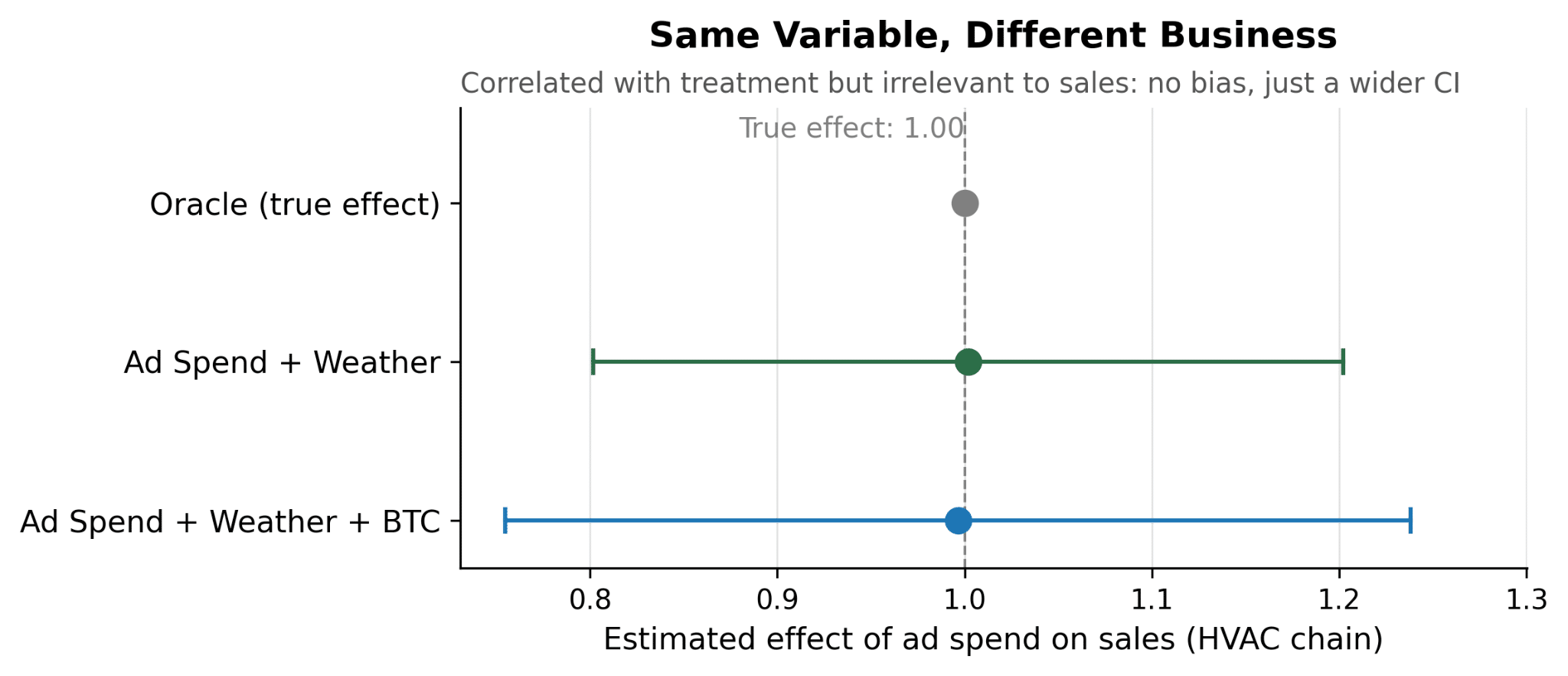
Both estimates land right next to the true incremental ROI of 1x, so omitting BTC price doesn’t bias anything here because BTC isn’t on any causal path to HVAC sales — it just moves along with ad spend. But the second confidence interval is roughly 20% wider.
When two regressors move together but one of them doesn’t help explain the outcome (here, sales), the model still tries to split some credit between them, and that attempt eats into the precision of the effect you actually wanted to measure, without improving the model. So there’s no silver bullet for what belongs in your model: variables themselves don’t tell you their role!
The Takeaway
Before including a variable in your model, ask one question: what role does it play?
- Confounders → include. They remove bias by accounting for shared causes of treatment and outcome.
- Mediators → exclude. They sit on the causal path. Including them blocks the effect you’re trying to measure.
- Colliders → exclude. They are caused by treatment and outcome. Including them manufactures associations that don’t exist.
These three roles are universal, but the variables that play them are not. For a crypto exchange, BTC price is a confounder, for an HVAC chain, weather plays that role, and for an egg brand, it’s stockout rates. There’s no generic list of variables to include in your model — only a generic method for deciding.
If you can’t articulate why a variable belongs in your model — what causal role it plays, which path it blocks or opens — it probably doesn’t belong there. When in doubt, draw the causal diagram first. It doesn’t need to be perfect. It just needs to make you think about what causes what before you start adding columns to your regression.
Variable selection is not a statistical question. It’s a causal one. Treat it that way.
Want to replicate our analysis?
The full R and Python scripts are available at https://github.com/getrecast/bad-controls