
Multicollinearity is one of the hardest problems in marketing analytics. If you took a statistics course in undergrad, you might have covered it; it describes a phenomenon where two or more variables in a model are correlated.
Let’s bring it to marketing to make it more tangible. Imagine we’re trying to analyze the impact of television marketing. We would go back and observe how television advertising varies over time and how it affects revenue.
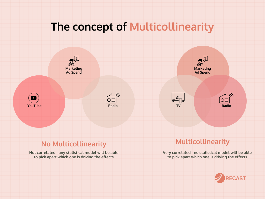
However, what if television and radio ad spend are correlated? Every time we increase spend on television, we also increase spend on radio by the same amount. This correlation creates a problem in our analysis because we’re unable to discern whether it’s TV or radio ad spend generating that extra revenue.
When you have two or more channels that are perfectly correlated, no statistical model will be able to pick apart which one is driving the effects – statisticians call this problem multicollinearity.
This can lead to inaccurate performance evaluation and suboptimal decisions about budget allocation. It increases the variance of the coefficient estimates, leading to wider confidence intervals or less precise estimates.
In practical terms, multicollinearity makes you blind and the range of possible incrementality becomes too broad to make confident decisions. This article will help you identify when you are experiencing multicollinearity and what you can do to solve for it.
Detecting Multicollinearity in Marketing Data
This is a very common problem: marketing teams often up or lower their budget across all channels at the same time. It’s also very common with seasonality. Knowing where and when you’re experiencing multicollinearity is the first step to fixing it. There are three main ways you can audit it:
A. Correlation Coefficients
One preliminary method to detect multicollinearity is examining the correlation coefficients among the predictor variables. A correlation coefficient of 0.8 or above typically indicates high multicollinearity.
B. Collinearity Diagnostics
Modern statistical software packages, such as R, Python’s scikit-learn, and SPSS, offer collinearity diagnostics during regression analysis, providing measures like Variance Inflation Factor (VIF), Tolerance statistics, and Condition Index.
C. Factor Analysis
Factor analysis serves as another tool to spot multicollinearity. This statistical technique seeks to identify underlying variables, or factors, that explain the pattern of correlations within a set of observed variables.
Overcoming Multicollinearity With Bayesian MMM
Traditionally, multicollinearity has posed significant problems for simpler analysis methods like linear regression. In such models, one variable may be randomly chosen to receive all the credit, while another may receive no or negative credit, leading to inaccurate results. If you only run traditional linear regression, you might even see results that show a negative impact on marketing spend, which shouldn’t be possible (for >99.9% of situations).
However, we now have more sophisticated modeling approaches to tackle this issue. Bayesian statistical methods, for example, can help better manage the problem of multicollinearity. Instead of randomly attributing credit to one variable over another or attempting to pinpoint which marketing channel was more effective, the model represents a level of uncertainty about the effectiveness of both channels.
Between two correlated channels, the model communicates that while it’s uncertain which channel drove more sales, it is confident that at least one of them did. This ability to provide an uncertainty range instead of incorrect attribution is a key advantage in sophisticated models like Bayesian ones.
That’s what we use here at Recast. This approach helps accurately quantify and communicate the uncertainty around the effects of different marketing channels on sales, even when those channels are highly correlated. Multicollinearity generates uncertainty in our estimates, but not bias.
Proactive Measures to Break the Multicollinearity Cycle
While Bayesian models offer an improved solution to handling multicollinearity, there’s another aspect to consider. The multicollinearity problem primarily pertains to retrospective analyses. However, marketers have the power to break the correlation moving forward.
If a company needs to determine the effectiveness of radio versus TV advertising, it can design a marketing plan to separate the spending on these channels. One month could involve heavy TV advertising with limited radio ads, while the next month could follow the opposite pattern. This divergence allows the company to observe changes in revenue linked to each specific channel, helping break the correlation and reduce multicollinearity.
You need some amount of difference in the inputs in order to be able to get an actual signal on how they are impacting the outputs. This strategy of proactive marketing channel manipulation helps break the correlation between channels and injects more signals for our model to better estimate the incrementality of each channel individually. While understanding historic multicollinearity is very complex, present and future collinearity can easily be solved for.
Conclusion
Multicollinearity is a significant concern in marketing mix modeling. While advanced modeling techniques like Bayesian methods substitute bias for uncertainty, the power to break the cycle of multicollinearity is in the hands of marketers – you have control over it.
As we continue to build Recast, there will be even more suggestions and recommendations that marketers will be able to follow to give the model even more certainty and, more importantly, for them to gather the data and insights they need to make their spend more efficient.