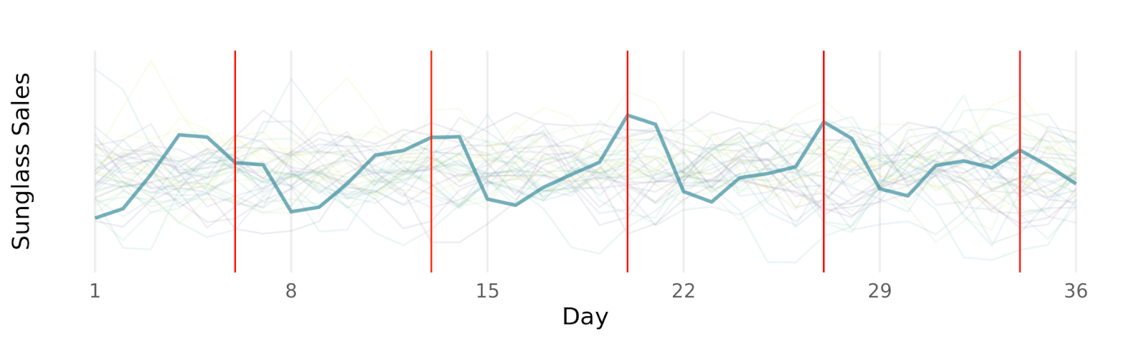
Time series data is special because the order in which observations occur is meaningful. For example, looking at sunglasses sales at Sun-Glasses-For-All (an imaginary brand), we can see that knowing yesterday’s sales gives you information about today’s sales. And sales this time last week gives you information about today’s sales (sales tend to peak on Thursdays as people prepare for the weekend 😎)
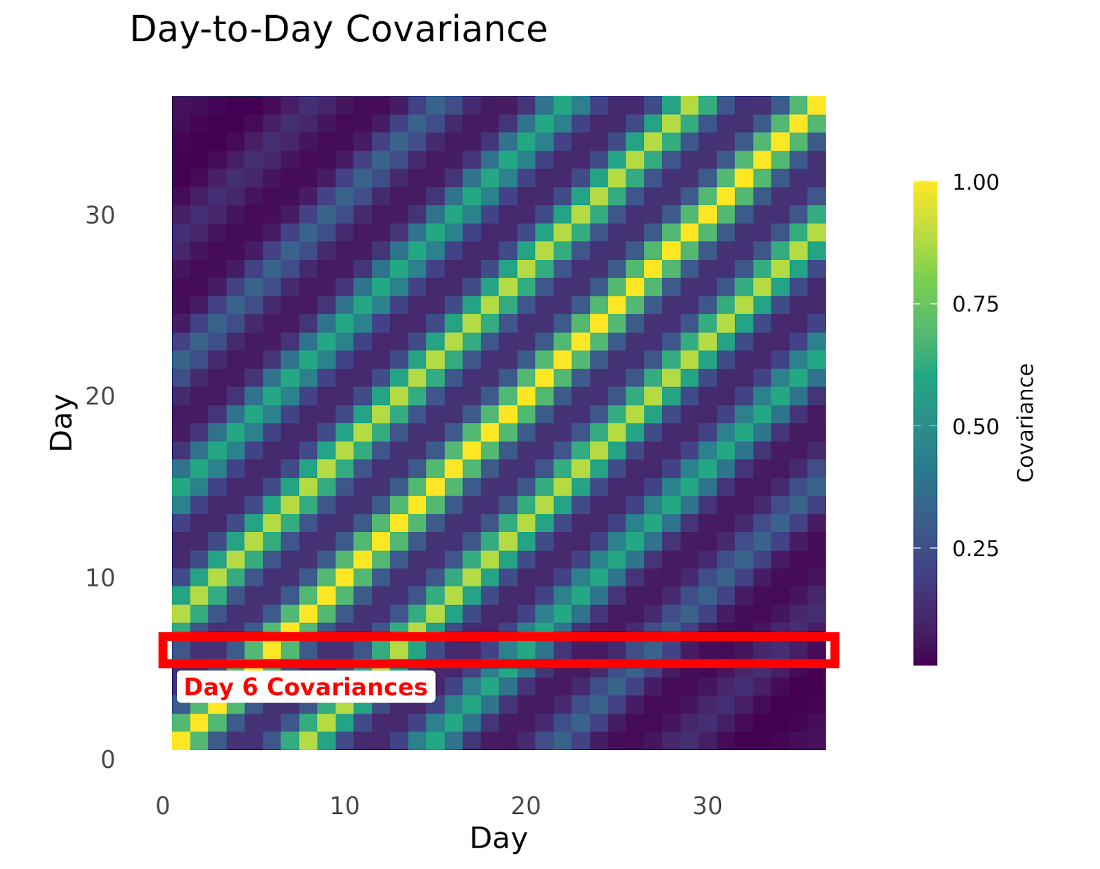
One way to encode that information about a time series is with a covariance matrix. Each cell in a covariance matrix tells you how two time points are related. Here, lighter values mean the row/column time points are very related, and darker mean the row/column time points are unrelated.
Here’s the covariance matrix for the sunglasses sales above. You can see that each day (a row of the covariance matrix) is highly related to the same day each week (Thursdays are similar to other Thursdays, but less so as time goes on) and each day is similar to the 1-2 days before and after it.
And below, we show the sales data and the covariance matrix where sunglasses sales are completely independent, every day has no similarity to any other day, even the days immediately around it. In this case, knowing today’s sales tells you nothing about the sales on any other day.


Finally, we show the sales data and covariance matrix where each day is related to the 2 days before and after it. You can see that while sales go up and down almost randomly, it does so more smoothly, making small changes each day as the effect of previous days decays.


So we can see that the covariance matrix is a way of summarizing the underlying patterns in time series data, which can be very useful for building more complex statistical models using time series data. So if you can learn the covariance matrix for a time series, you can use that matrix to make better forecasts into the future!
One important use for these types of covariance matrices is that you can use them to build a bayesian statistical model where you encode a lot of useful prior information about the likely relationship between time points by thoughtfully choosing the structure of your covariance matrix. Like Sun-Glasses-For-All you might know you have strong yearly seasonality because you know that sales peak in the late spring and fall in the winter.
Having a covariance matrix for your time series helps explicitly outline how different time points are related to each other, which can help you understand trends that occur in your data.
Kernel Functions
Defining the covariance matrix allows you to understand how timepoints are related. But what about future timepoints that have not been observed yet? At Sun-Glasses-For-All, we’re about to set our revenue forecasts for the next 2 years in order to allocate budget and plan needed upgrades to our business. A covariance matrix looking at the last 3 years of data plus timepoints 2 years into the future would be at least an 1825×1825 matrix . That’s over 1.5 million unique covariances between days to consider.
Rather than explicitly creating covariance matrices element by element, considering each day’s impact on all the other days, we can use a kernel function which takes in two time points, and spits out their covariance according to a structure we define. We no longer need to explicitly think about and define the relationship between today’s sales and sales on March 5th 2 years from now! The kernel function will calculate it for us, based on the structure we give it.

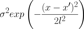
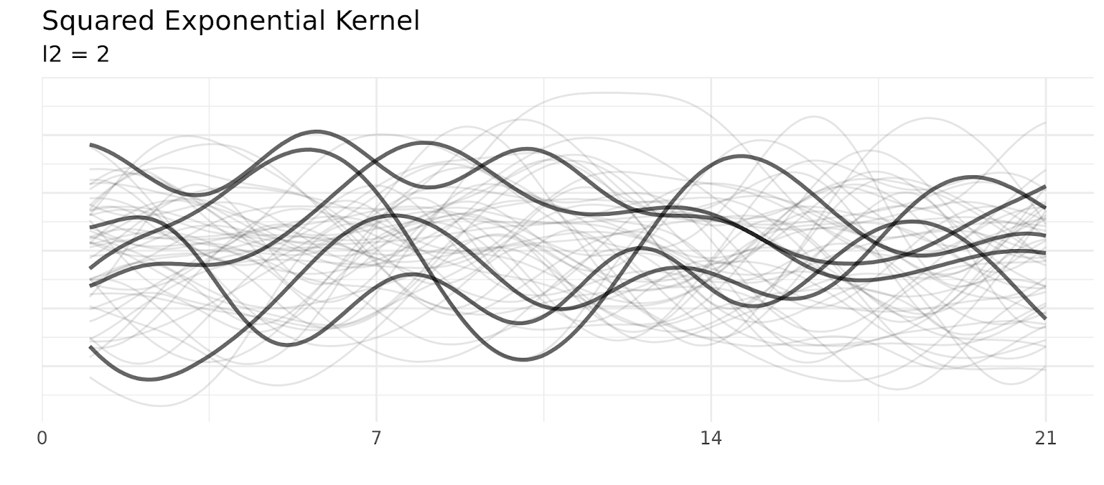
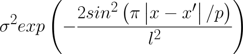
For example, a kernel called the squared exponential kernel uses this formula to define the relationship between two points:
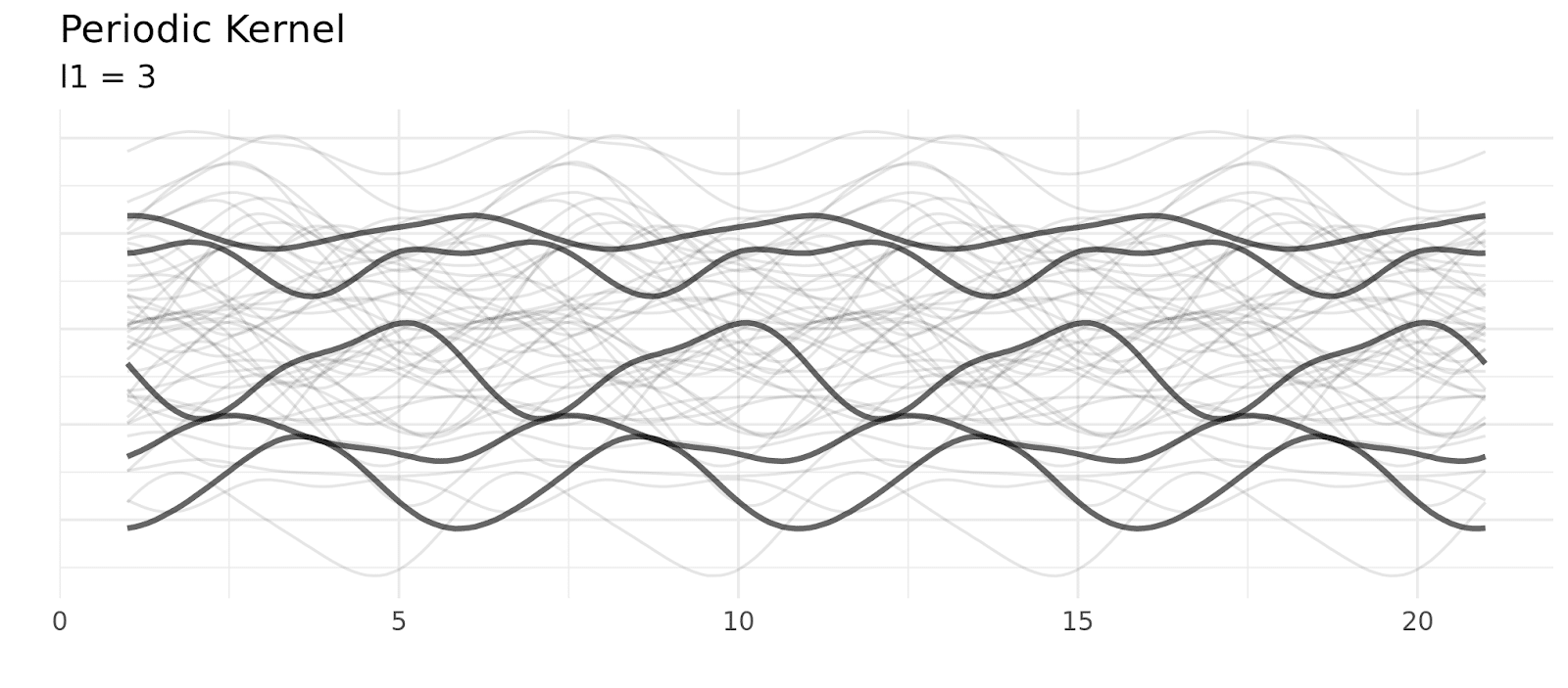
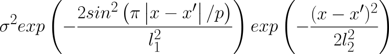
And a kernel called the periodic kernel uses this formula to define the relationship between two points:
A common kernel called the locally periodic kernel combines the squared exponential and period kernel (by multiplying them) producing a kernel that still has periodic elements, but allows those elements to change over time.
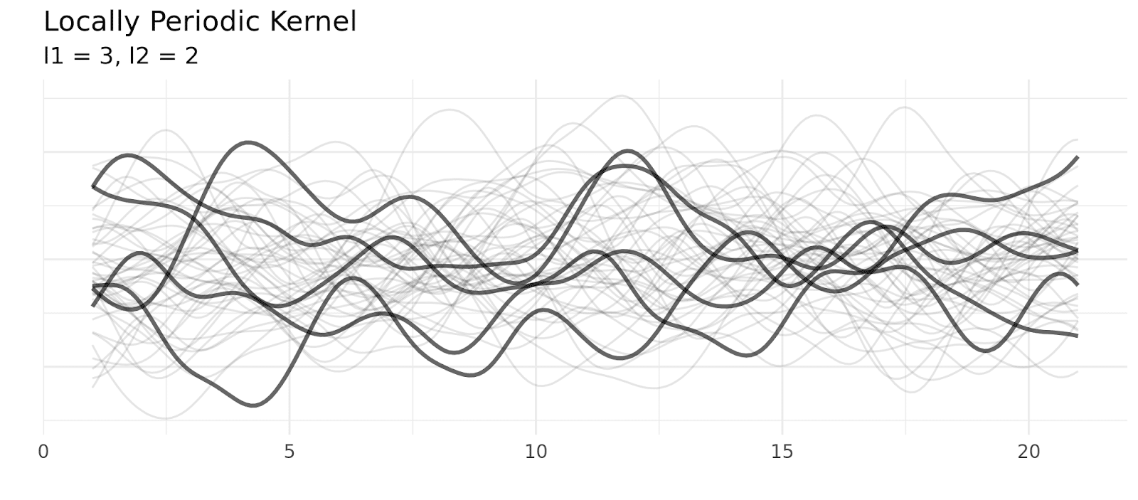
When you choose a kernel, you’re giving the model a prior about the structure of your time series. Is it smooth (changes happen slowly over time?) Is it periodic? (Today’s sales tell you a lot about sales this time last week, or this time last year?)
Choosing a kernel allows you to leverage knowledge you have about your time series and restrict your time series to shapes/patterns that are reasonable. For example, if we’re using a Gaussian process to model how the baseline ROI of Sun-Glasses-For-All’s TikTok campaign changes over time, we can choose a kernel that accurately captures the seasonality (more effective in the summer than the winter) and smoothness (given that we’re not making wild swings in our strategy, we expect baseline ROI to make smooth changes rather than wild jumps). These configurations also help you understand the future of your time series: if we can accurately pick up on seasonal patterns with a seasonal kernel, we can plan better for next summer, and the summer after that.
Fitting a Gaussian Process
There are two sources of information in the Gaussian Process model:
- the kernel (and covariance matrix) of your model gives your Gaussian Process model useful prior information on the way your sales change over time
- the observed data (like your last 3 weeks of sales data) gives your model useful information about which prior samples are reasonable given the data you’ve observed
Whereas before, the covariance matrix we created using our kernel could generate a whole plethora of sales numbers over time, now we can whittle that set down to only sales values that are similar to our observed sales data.
Mathematically, we do this by conditioning our covariance matrix on the observed sales data. In other words, the model whittles down the prior time series samples into ones that make sense with the data you’ve observed.
This takes our reasonable sales data from these samples…
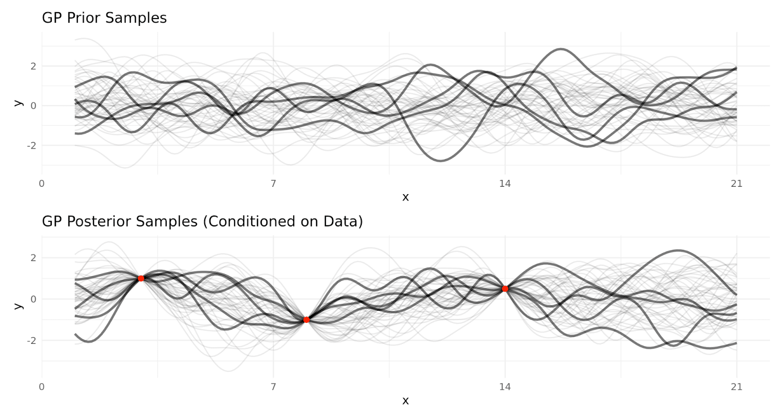
…to these. You can see in the bottom pane, the only samples allowed by the Gaussian Process are ones that align with the observed data (red dots).
And at its simplest level, that’s how you fit a Gaussian process to time series data!
- Use your expertise to select a kernel (or multiple kernels) that describe the way the timepoints in your data are related to each other so that the model knows what a “reasonable” time series looks like in your context
- Add in the data you’ve observed so that the model knows which of the many “reasonable” models best fit the data we’ve already seen
Samples and Uncertainty
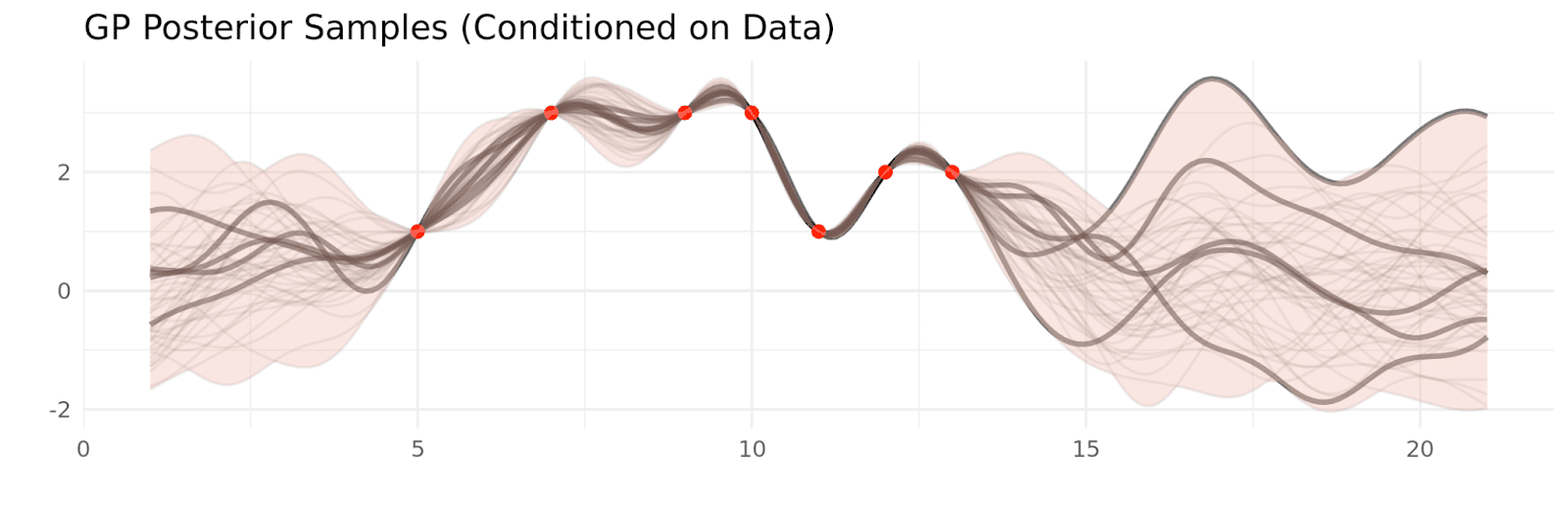
While conditioning on real data narrows down the samples to those that are compatible with our data, there’s still a lot of variability, especially when there’s not a data point nearby. This makes sense, if we haven’t observed recent data, we’re not really sure what’s going to happen. Having variability is great because it allows you to quantify how certain your predictions are, and make decisions with that in mind.
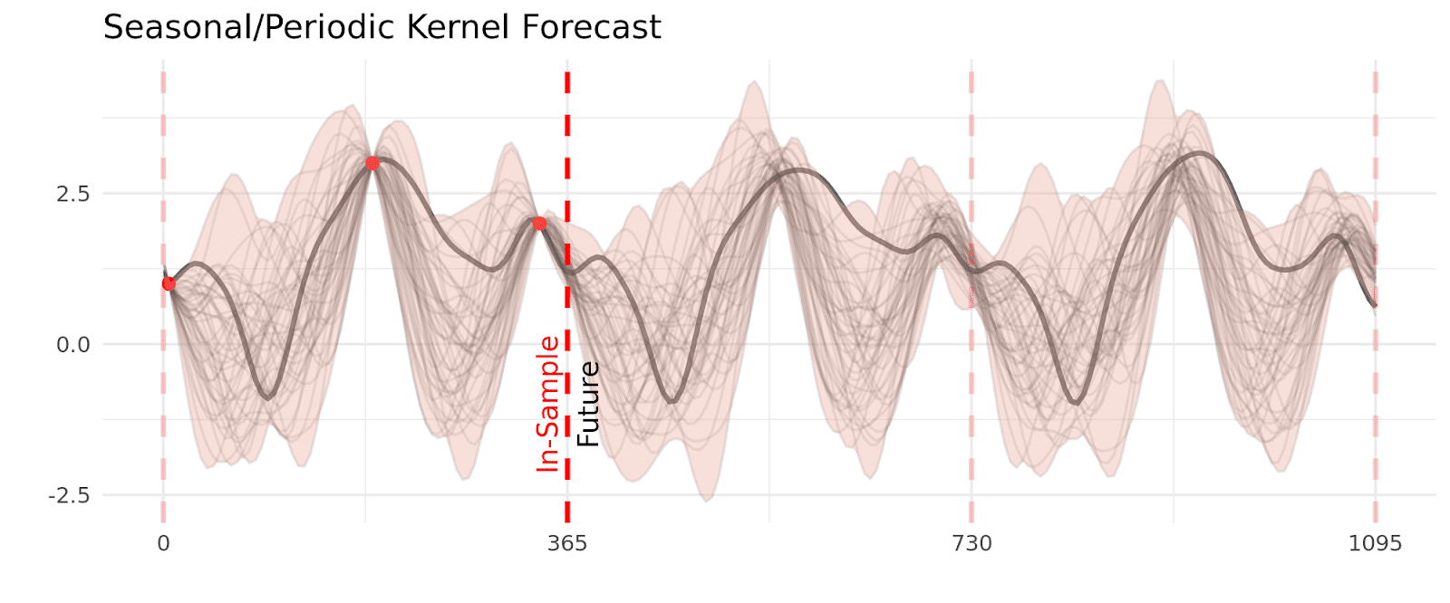
While we can use gaussian processes to forecast far into the future, you’ll notice that the kernel you choose impacts the usefulness of this forecast. By definition, forecasts look at time points that do not have observed data nearby, so we rely on longer term relationships, like seasonality. If your kernel includes yearly seasonality, then even though the smooth component may age out of the model quickly, yearly seasonality can still shape the forecast years into the future. Similarly, the stiffer your kernel (it changes very slowly over time) the longer your observed data will impact your forecast.
Conclusion
While it is not the only application, Gaussian Processes are a powerful tool for modeling things that vary over time. At Recast, we use Gaussian Processes to model time-varying parameters like channel efficiency, and organic sales/conversions.