
TLDR:
- Recast’s research team made model fitting for our Bayesian MMM 5-20x faster and reduced the median runtime from hours to just minutes. We’ll explain how in this article.
- Runtimes limit how quickly you can deploy a model and how many iterations you can make before a strategic review. So if a model runs in 10 minutes, for instance, you can question a result, change an assumption, and rerun it before it gets put into action.
- Although our code is written in Stan, the ideas we used to accelerate Bayesian MMM fitting also apply to Python and R, so a lot of the discussion below will be helpful to practitioners more broadly.
When Michael K and I started Recast, fitting an MMM was often a multi-day commitment. We’d leave our computers humming, come back the next morning, and often find that the model broke somehow and that we had to start all over again.
We’ve come a long way since then, but every so often we still get asked why Recast models take a long time to fit. It’s a fair question! And the implication behind that question is that we’ve built something needlessly complex. MMM doesn’t involve much data, after all – typically two years of daily spend and KPI data across twenty channels or so – and you can fit a regression to it in a few seconds.
Only we don’t fit a regression at Recast. Doing so would mean asserting things about how marketing performs that we simply don’t believe. Like saying a channel’s ROI was the same in 2024 as it is now, or that a single number can encompass how fast an ad’s effect decays or where that channel saturates, or that a point estimate without uncertainty is enough to make decisions with.
We don’t believe any of this is true. So in Recast, ROI can vary over time, every channel gets its own saturation curve, holidays and promos are allowed to have their own shapes, every estimate comes back with its associated uncertainty, and so on. So a twenty-channel Recast model carries something like 30,000 parameters, and fitting one means the model evaluates itself against the data roughly 250,000 times.
That’s why Recast was “slow”. We demanded a model that we felt adequately captured how marketing really works.
Which brings me to some good news.
Rok Cesnovar and Drew Schmidt on our research team have made Recast 5–20x faster. Our median runtime is now just 14 minutes, down from 3.5 hours on massive compute (not on a laptop!). And that did not require simplifying the model, loosening any priors, or dropping any parameters. We simply went down to the bones of the model itself and found ways to stop wasting computational time.
Our research team found these savings in four key places, and none of them are particularly glamorous on their own: Stan’s general-purpose gradient machinery, which we replaced with gradients derived by hand for our specific model; an inefficient memory layout; independent calculations running in sequence for no particular reason; and tens of thousands of intermediate values being written to disk that were not needed downstream. I’ll walk through each of these areas below.
But before we do that, I want to pause and say that what I care about most here isn’t really the headline runtime number, but what it means for our customers. Fourteen minutes is a short enough runtime to quickly rerun a model if something looks off. It means our team can iterate faster during the model-building phase. And soon, it will mean our customers can change their model’s assumptions and rapidly see how those changes impact their forecasts and marketing plans.
First, why does fitting an MMM take so long?
Let’s backtrack for a second and consider the scope of the challenge here.
The input data for an MMM is usually spreadsheet-sized, perhaps two years of daily marketing spend by channel and your KPI, yet fitting a Bayesian model to that history can take many hours. This makes each attempt costly in terms of both computing resources and time. Model builders need to wait between iterations and end users of can face long waits before their models are delivered.
Long runtimes are largely the price to enter of Bayesian inference. For example, a typical Recast model estimates roughly 30,000 parameters from about 730 daily observations (or two years of marketing data).
At that ratio, many different combinations of those parameters explain a brand’s marketing performance equally well. One combination might put a large channel’s incremental ROI at 1.2x, and another at 3.4x, and both fit the data about equally well. The data alone does not pick between these paths, so the model has to carry all of them rather than pretend one is the answer.
That’s what the model sampler is doing while you wait. At each iteration, it evaluates how well one combination of parameter values explains the observed data, then follows the local gradient to decide where to look next. It runs thousands of iterations, each one a full pass through the model.
It’s definitely slow, yes. But the alternative is a single point estimate of marketing performance with no honest account of the other outcomes consistent with the original dataset.
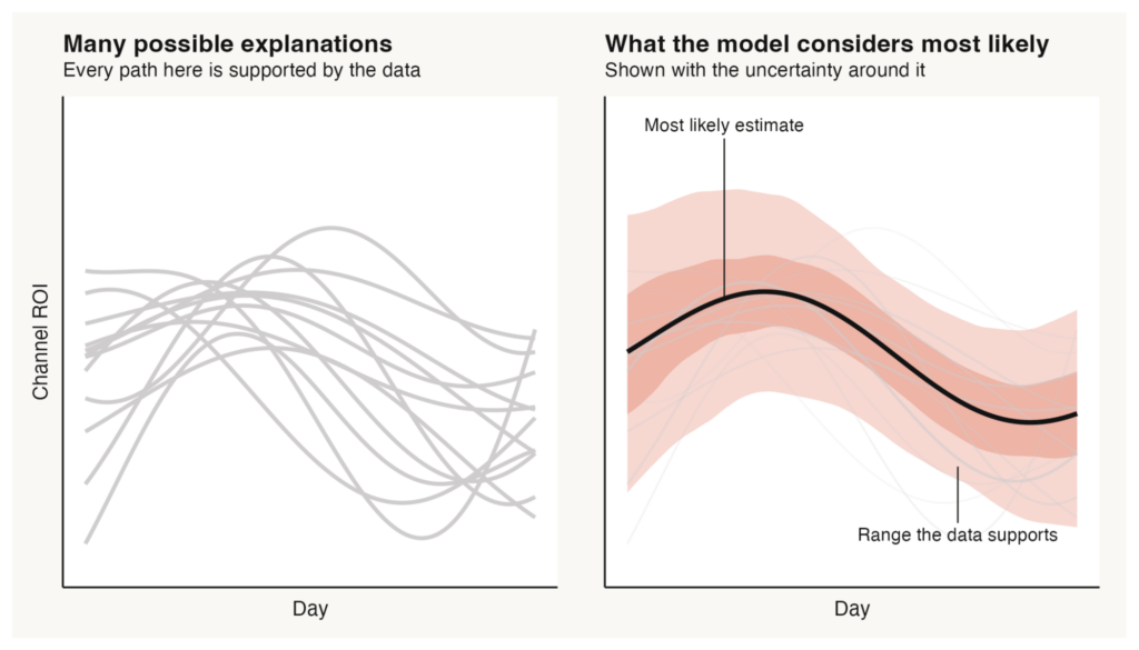
Below there’s an illustration of what this search roughly looks like. On the left, each gray line is a possible path of a channel’s ROI that the data can support. On the right, the model reports its most plausible performance estimate and the uncertainty around it.
Yes, MMM can be slow. But our research team spent the last few months focused on where the time actually goes when we fit a Bayesian model. And they found there are two routes to a shorter run:
- The model can take fewer, more efficient steps to find plausible explanations for a given dataset, reaching the same trustworthy answer after evaluating fewer possibilities, or;
- Each remaining step can also be made less costly for instance, by eliminating repeated calculations, organizing data for faster access by the processor, and running independent work in parallel.
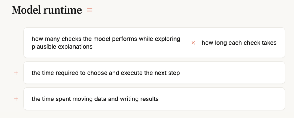
So a useful breakdown of a model runtime separates the cost of searching, choosing and executing the next step, and then writing data so we can see where each optimization can help.
How we actually reduced model runtime
In each step of the model fitting process, the model asks “If I nudge the parameters a little bit, does the fit get better or worse, and in which direction?” That answer tells the sampler which direction to choose. That’s why the first term, the number of checks multiplied by how long each one takes, dominates the other two terms of the equation.
Our researchers Rok Cesnovar and Drew Schmidt went straight to the most expensive part: calculating how a small change in each parameter would affect the model’s fit. The tool behind it is called a gradient, the same one used to train artificial intelligence, which tells the model whether the fit would improve or worsen and in which direction.
Stan’s general-purpose functions can calculate gradients for many kinds of models, but that flexibility comes at the cost of extra work. Because we know the mathematical structure of Recast models, our team wrote specialized Stan functions from scratch that compute gradients directly. These “analytical gradients” answer the same question about which direction the model should go, but with fewer operations each time.
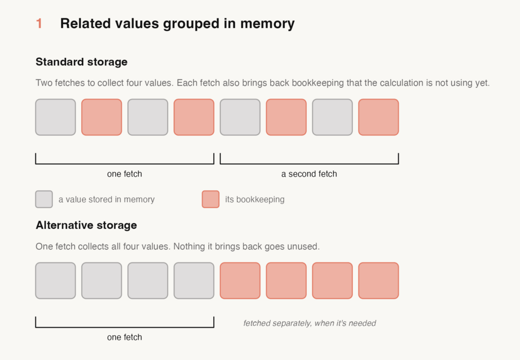
Writing our own specialized Stan functions also let us organize data more efficiently in memory. Normally, Stan stores each value next to extra information it will need later to calculate gradients. But processors retrieve memory in blocks, so when the calculation asks for several related values, it also pulls in a bunch of that extra information we may not need – very inefficient!
We separated the two instead, putting the values together and the gradient-tracking information somewhere else. That way, the processor can grab one continuous block of the data it actually needs, without bringing along unnecessary information. The illustration below shows this.
Another runtime optimization is to perform more computations simultaneously (called “parallel processing”). A lot of the calculations involved in fitting a model don’t depend on one another, so there’s no reason to make the processor finish one before starting the next (called “sequential processing”).
Say you have four independent tasks. If you run them sequentially, the total time is the sum of the time spent on all four. Run them in parallel, and you’re mostly waiting for whichever task takes the longest. The next figure shows the difference between the two approaches.

And the last optimization is actually pretty simple: don’t save data you’ll never use!
A standard model run can generate a huge amount of intermediate output data. So we rewrote Stan’s functions to keep the results we actually need, throw away the rest, and save what remains in a compact format. In one part of the process, for example, we need about 80 values. A standard approach would write more than 50,000 values to disk and then read them back later. Avoiding all of that means moving less data around and skipping work that has no impact on the answer we’re looking for.
Imagine all of these changes together, and then imagine the speedup gains:
- Model-specific gradients make each calculation cheaper and let us organize related data more efficiently in memory.
- Hardware-aware calculations and parallel processing cut down the work in different ways.
- And once the model finishes fitting, selective output keeps us from wasting time saving and reloading results we’ll never use.
None of these changes affect the statistical question we’re asking. They just help the computer get to the same answer, with the same uncertainty quantification, while doing a lot less unnecessary work.
What faster model runs make possible
This is all pretty fascinating for technically minded readers, but what do we achieve beyond speed for its own sake? With faster-running models, you get more chances to question them before you commit to a decision. You can look at the result and ask:
- “Does this actually answer the business question?”
- “Does anything look weird?”
- “Should we change an assumption or try a different specification?”
And because another Recast run is relatively cheaper now, you can test that idea instead of committing to the current “good enough” version.
You can also compare several versions of the model rather than committing to the first one that works. Test different assumptions and see whether they change the recommendation. This can look like:
- Running the model with shorter and longer carryover windows, then seeing whether it still recommends the same budget.
- Or maybe you are unsure whether a sales spike came from marketing or a promotion, so you account for the promotion in one run, leave it out in another, and compare the result.
Then you can incorporate that information and run it again!
Faster computation can also let you ask a bigger question. Maybe you want to include more marketing channels in your models or estimate them across more geographic regions. Those decisions are more accessible with dramatically faster runtimes.
So it’s the consequences for customers that I really care about with these performance improvements. A 14-minute median run and a 5-20x speedup do more than save our team a few hours. They give our users more chances to challenge an assumption, compare alternatives, incorporate something new, and catch a problem before they move any marketing dollars.