
How to use this article:
- This is a practical guide for both technical and non-technical practitioners. No prior statistics background is required.
- Throughout the article, you’ll find short embedded videos that walk through key concepts visually. We recommend watching them as you go.
- If you’d like to follow along with real code and run the examples yourself, we’ve published an open-source companion repository here: https://github.com/getrecast/public-recast-code-examples
- The repo includes reproducible examples in R using simulated data so you can see multicollinearity (and the methods to handle it) in action.
While preparing for your work day, you start to make your morning coffee and realize you’re completely out of grounds. Worst day ever. Now you need to figure out the fastest way to get from your home to the grocery store and back again so you can get your caffeine fix before a headache sets in.
Naturally, you’ll consider the distance, the number of traffic lights, where traffic is likely to be, if the traffic will be worse at certain times of the day, and so on. As you consider these things, you start to realize that they are all interconnected:
- Routes with longer distances often have more traffic lights,
- Heavy traffic usually occurs around rush hour,
- Speed limits tend to be higher on longer routes (e.g. you’re taking a highway).
So what really matters? Is it the distance? The speed you drive? The number of traffic lights?
This is the problem of multicollinearity and it has huge repercussions for end users of media mix models – more on that in a minute.
First we need to handle this coffee example! If your goal is to arrive at your destination as quickly as possible, these factors are often redundant; for example, picking the shortest distance will give the same result as picking the route with the fewest number of traffic lights (since shorter distances probably have fewer traffic lights).
Let’s break this example down a bit further before applying this understanding to the context of marketing measurement. Consider the following simple equation:

As distance increases, so will your time of arrival. But so does the number of lights that will interrupt your commute. So, in this equation, if distance and the number of lights are perfectly correlated with one another (e.g. for every mile, you get one additional traffic light such that a 4-mile commute would have 4 stoplights), the time to arrival is influenced identically by distance and the number of lights. Think of it this way – if the distance in miles is always equal to the number of traffic lights, then your measure of distance and traffic lights are identical – it’s just that one value, distance, is measured in miles/km while the other is measured as a discrete count!
In a standard linear regression equation, which attempts to estimate an outcome based on predictors, this creates a frustrating mathematical result. Since the values of distance and the number of traffic lights are identical, so too is their relationship with your time to arrival. This means that our predictions for time to arrival are equally accurate when using distance alone or traffic lights alone.
Let’s look at a practical example to help this make more sense. Imagine that you collect data on your morning commute for a month and that you live in a meticulously constructed neighborhood – we’ll call it TrafficTown – in which there are 2 traffic lights per mile. No matter which route you choose to take in TrafficTown, the number of traffic lights will always be equivalent to the number of miles traveled times 2. The data you collect on your commute looks something like this:
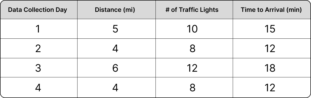
Using these data, we deploy a regression equation to solve for the relationship between distance, traffic lights, and our commute time. You ask the equation to tell you how long it will take you to commute based on the distance of your commute and the number of traffic lights you encounter. The equation spits out highly reliable, accurate predictions that are statistically significant (meaning they are unlikely to be the result of random chance). That’s great news! But when you take a closer look at your regression equation, you see something weird:

What’s going on here? The regression equation is telling you that the coefficient for traffic lights is 0. In other words, traffic lights don’t seem to have a meaningful impact on your arrival time. You rightfully shake your head in dismay and think, “perhaps this is a bug. I’ll rewrite the equation with traffic lights first. That’ll fix things.” But your regression equation misbehaves again in exactly the opposite way.

At this point, you might be wondering if you’re really cut out for this whole statistics thing. Should you just throw in the towel? No!
Take a look at these equations and use some of the values in the table above to solve for time to arrival. The equations are equally accurate in outputting the correct time to arrival. Even though one equation reduces the traffic light coefficient to 0 and the other reduces the distance coefficient to 0, both are able to represent the data with the same level of accuracy!
So which of these two equations should you choose? Functionally, neither make any practical sense. And since you really need to get to work on time, what you ultimately care about is what is causing changes to your commute time in TrafficTown. Of course the number of traffic lights impacts commute time, we can’t ignore those. And what kind of arrival time prediction would we be making if we left out distance? It’s not that we’re fundamentally misunderstanding how our commute works, it’s the way the regression equation is structured that is driving this impractical result. Inferring the cause of changes to our commute time using only a regression equation like this one, therefore, is practically impossible.
The important point here is that regressions are not magic truth-telling machines, despite the temptation to treat them as such in marketing measurement.
Just because you “control for” all of the variables that might cause a change in your commuting time doesn’t mean that you’ll get correct estimates for the true impacts of those variables – just imagine how much worse this problem would become if we attempted to consider an even larger number of predictors (e.g. number of turns, gallons of gas consumed, etc.) that are inherently related to one another! The results would quickly become unusable.
Applying this Learning to Marketing Measurement
Now, let’s bring this challenge back to the realm of marketing measurement. In the equations above, time to arrival represents your marketing KPI (e.g. revenue). The distance and traffic lights in TrafficTown represent your spend in various paid media channels. And that multiplication (the coefficient) for each represents the proportion of spend that becomes revenue (your ROI).
So, we could restate the equation like this:

This equation is a simplification of a typical marketing mix that has dozens of channels, but hang in there.
If spend in Channel A is totally independent of spend in Channel B, this equation will work just fine. But what if they aren’t? What if the spend in channel B is dependent on the spend in channel A such that as spend in A goes up, so too does spend in B? Consider this iteration of the equation above:

This happens all the time in marketing. You may, for example, have a top-of-funnel (TOF) strategy in which you increase spend in linear TV and connected TV (CTV) simultaneously to capture some seasonal demand in your business. The question, though, is which channel is actually driving incremental revenue? If you spend across these channels in lock step (for every $4 increase in linear TV, you increase spend by $1 in CTV), you’ll run into the very same problem as our work commute example above!
The “credit” for driving incremental revenue will go to either linear TV OR to CTV because the total revenue generated can be explained by either. And, if revenue is explained by one paid media channel, that means the other paid media channel must evaluate to 0 to retain an accurate prediction of your revenue. That would look something like this:

But the model would fit the data just as well if we stated the equation like this:

For practitioners using these marketing models to guide budget decisions, disparities in output that “explain” the KPI (like the CTV vs. Linear TV disparity above) can have serious implications on where media dollars get allocated (or misallocated).
At this point, you may rightly ask, “Why doesn’t the equation split out the revenue impact proportionally?” Well, for the same reason that we don’t account for the traffic lights in the simple commuting example above. The equation can explain the top-of-funnel revenue outcome using just one channel OR the other, but it won’t be able to use both in a simple regression equation like this one when the channels are fundamentally collinear. This further inhibits our ability to identify the marketing driver of incremental revenue. Since our ultimate goal is to identify which channels are causing increases in revenue, we’re stuck!
Standard linear models will always suffer from this issue with strongly correlated channels and the result for marketers is often an inability to make agile, robust decisions with modeling outputs. The example above is a simplified one, but the core learning remains – collinear channels, those that move in lock step with one another, are likely to have unreliable and inaccurate efficacy measurements in simple linear models of marketing performance. This presents real challenges for marketers who are trying to use their output to guide high-stakes budget decisions.
Reduce Multicollinearity via Intervention
Many marketers using advanced measurement methods like MMM aren’t aware that multicollinearity could be skewing their results. Or, recognize the issue but don’t know what to do about it. But not you! This problem of multicollinearity is not a fatal one and is within your control to manage through simple, practical steps that will help your model find stronger signal and make more accurate recommendations for where to allocate your marketing budget.
If you suspect correlated spend patterns might be limiting your marketing model’s ability to isolate the incremental impacts of paid media channels, you can introduce intentional variability into your spend strategy to help reduce the impact of multicollinearity in your models. Here are a few practical spend strategy steps you can take to increase the signal given to your model and reduce the impact of multicollinearity:
- Running A/B tests, Geo-based tests, and lift/incrementality tests can also provide strong signal and help you better identify a channel’s true performance. These learnings can then be integrated into your modeling approach.
- Intentionally throttle spend in channels with similar strategies. Spend a little higher on linear TV this week and then pulse up CTV the following week.
- Go dark, one at a time, on channels that you suspect could be collinear. For example, go dark in Meta Prospecting for two weeks, then turn it back on before turning TikTok Prospecting off for two weeks.
- If you have a highly seasonal business and do most of your spend during specific times of the year, consider flighting your spend both with and against your seasonality (e.g. spend down a little as your seasonal demand increases and spend up a little as it decreases).
For a number of reasons, the above recommendations may be unpleasant to consider. Perhaps you, rightfully, fear losing money by spending down during strong seasonal periods or you feel that there is a strong additive impact of running similar channel strategies simultaneously. These are real risks, but so is making high-stakes decisions with a marketing model that has failed to identify true causal relationships.
Handling Multicollinearity via Statistics
To be clear, there is no way to eliminate multicollinearity entirely. It’s an unavoidable reduction in signal that puts an absolute limit on what can be learned from the data. The best that we can do, from a modeling standpoint, is handle multicollinearity with various statistical transformations, each of which carry tradeoffs.
These statistical processes aren’t really eliminating multicollinearity, they’re just accommodating for it. Though statisticians have no magic wand to resolve this issue, we can make well-considered decisions on which statistical processes to use based on their inherent tradeoffs!
At Recast, we believe that in most situations the best way to handle the uncertainty introduced by multicollinearity is simply to embrace it. We want to propagate the uncertainty through the model so that everyone is clear about the true uncertainty in the model. Recast does this with a Bayesian approach (described below) but we can also examine a few other common approaches along with their tradeoffs.
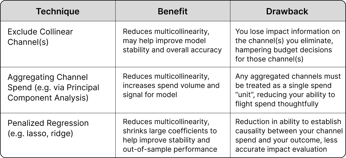
This, of course, is not an exhaustive list and there are a number of additional techniques that marketing analytics teams can use to help accommodate multicollinearity. However, one method, in particular, stands poised to provide many of the benefits highlighted above with fewer of the drawbacks: Bayesian inference. The Bayesian approach to handling multicollinearity is not to attempt to eliminate it but rather to quantify it by adding more uncertainty to collinear channels (to learn more about uncertainty, check out this article).
In the example above, we have spend in CTV and Linear TV moving in lock step. As a result, our Bayesian model will not be able to accurately assign “credit” to the correct channel in a consistent and reliable manner. So, instead, the Bayesian model reflects this with wider uncertainty around collinear channels. This is also probably a stronger reflection of reality. As John Wanamaker famously said, “Half the money I spend on advertising is wasted; the trouble is I don’t know which half.” This is, functionally, what the Bayesian model will suggest to you – we know that linear TV and CTV are impacting revenue, we just are uncertain about the level of impact across the two!
The advantage of the Bayesian approach is that we can quantify that uncertainty. This allows for more thoughtful scenario planning and can help marketers and modelers avoid being caught out by big coefficient changes in their models. To illustrate this difference, let’s use a standard (frequentist) linear model and look at the uncertainty produced by the outputs compared to a Bayesian approach:
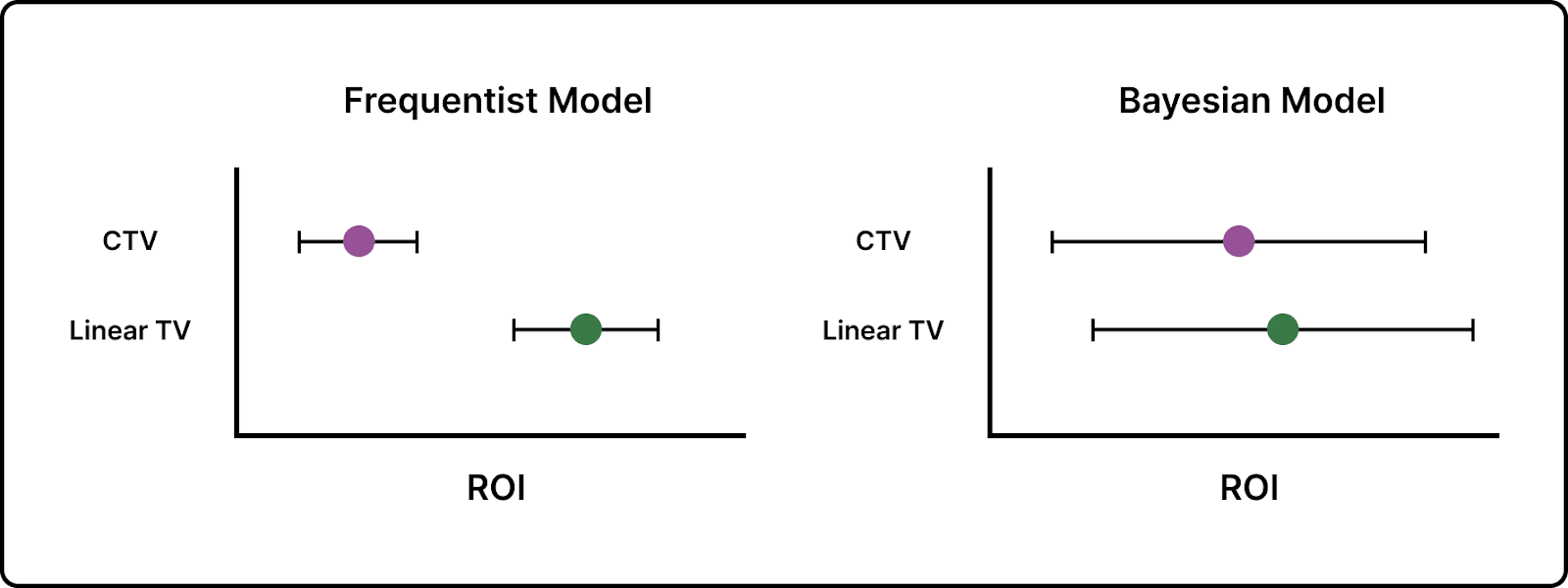
The frequentist model on the left assigns a much higher ROI to the Linear TV channel and a much lower ROI to the CTV channel. Those little tails represent uncertainty. So, overall, the frequentist model appears to believe, pretty strongly, that Linear TV is driving ROI. But what if the collinearity is creating a false positive? Remember, in a traditional regression like the frequentist model illustrated above, if credit goes to Linear TV, then the CTV ROI will tend toward 0 if those two channels are collinear. Since multicollinearity prevents a regression of this kind from finding accurate signal, both the ROI estimates and the uncertainty bands surrounding them are a misrepresentation of the true impact of your channel spend.
If you spend all your budget on Linear TV instead of CTV as a result of this recommendation from the frequentist model, you’ll be in serious trouble if collinearity is creating a false positive. The Bayesian model, on the other hand, shows similar ROIs between the linear TV and CTV channels with wide uncertainty bands. Where the frequentist model may provide you with false confidence that could lead you down the incorrect path, the Bayesian model more clearly describes the uncertainty you face as a result of collinearity and can help reduce the temptation to make big budgeting changes across collinear channels.
While this approach doesn’t guarantee the identification of a causal relationship, it is less likely to suggest such a relationship is present when multicollinearity is messing with your results. This can help you zero in on the actual causal relationship between your marketing spend and your revenue by helping you identify channels for testing and intervention without falling victim to false confidence provided by the results of a less sophisticated model.
Final Thoughts
Multicollinearity is a reality in marketing measurement that cannot be avoided. The best we can do as thoughtful modelers and practitioners is to be aware of its presence and take mitigating steps to ensure that multicollinearity doesn’t lead us down the wrong path (and into poor marketing investments).
Thoughtful marketing spend flighting practices can help and are the most effective method for handling multicollinearity. In addition to strong spend variation practices, statistical methods designed to handle these challenges – like the Bayesian approaches used at Recast – can further reduce the impact multicollinearity has on your marketing measurement.